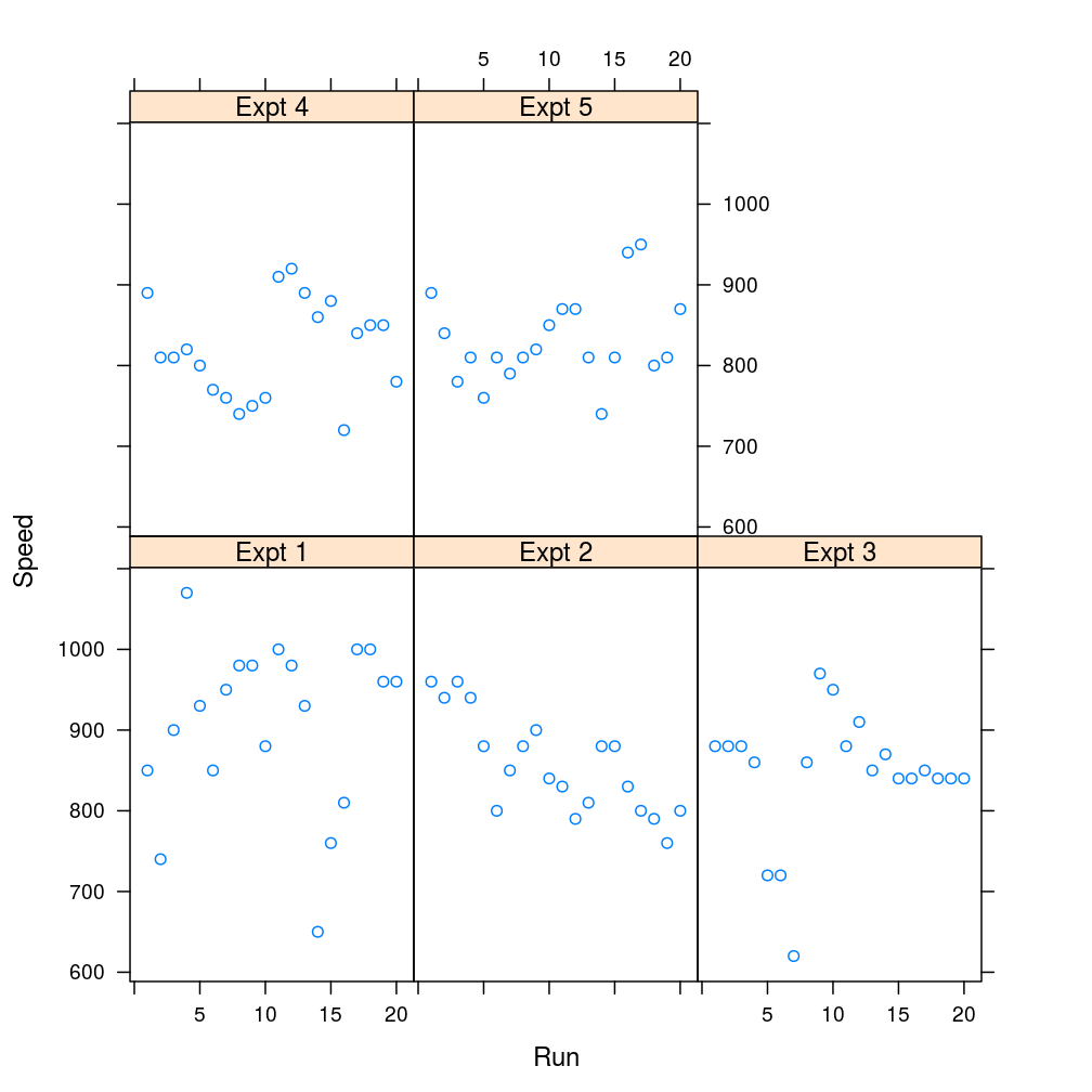
Graphic packages like lattice and ggplot2 work best when data are presented in long format as opposed to wide format into which data are typically imported and in which it is usually convenient to perform calculations. For example morley is a data frame in long format, which allows functions like lattice::xyplot to receive simple formulas and yet produce a complex trellis display.

library(lattice)
data(morley)

Take e.g. the formula Speed ~ Run | Expt, in which the speed of light measured by Michelson in 1879 plays the role of a response variable, the measurement run that of a predictor and the experimental replicate acts as a conditioning variable:

morley$Expt <- as.factor(paste("Expt", morley$Expt)) # adjustment for xyplot
xyplot(Speed ~ Run | Expt, data = morley)

So, how is a given data set to be restructured between the wide and long format? How do those structural properties reflect the underlying experimental design such as a longitudinal or a factorial one? And how to use stats::reshape, R’s principal restructuring tool with a given structure/design?

Basic structure of the wide and long format

To grasp the difference between the long and wide format, consider $m$ experimental units (a.k.a. records, observations, …) on which $n$ variables have been observed. We will distinguish among the $m$ units using ids $u_1,...,u_i,...,u_m$, and among variables with a set $\mathcal{V}$ of labels/classes where $\mathcal{V} = \{v_1,...,v_j,...,v_n\}$. It is helpful to regard such labels as generalized indices and any set like $\mathcal{V}$ a index set for variables (and not for units). In the morley data set ids are run numbers so that $u_1 = 1,..., u_m = m$, whereas variable indices $v_i$ are experiment numbers. However for most real-world data sets neither type of indices are integers (consider patient ids, for instance).

Our data set may be written as the statistical table

$$\begin{matrix} \text{id} & \text{var } v_{1} & \cdots & \text{var } v_{n} \\ 1 & Y_{1v_1} & \cdots & Y_{1v_n} \\ \vdots & \vdots & \ddots & \vdots \\ m & Y_{mv_1} & \cdots & Y_{mv_n} \\ \end{matrix}$$

It is this table that is modeled in R as a data frame in wide format. The long format, in the other hand, corresponds to the following table:

$$\begin{matrix} \text{id} & \text{var} & \text{index set } \mathcal{V} \\ 1 & Y_{1v_1} & v_1 \\ \vdots & \vdots & \vdots \\ m & Y_{mv_1} & v_1 \\ \vdots & \vdots & \vdots \\ 1 & Y_{1v_n} & v_n \\ \vdots & \vdots & \vdots \\ m & Y_{mv_n} & v_n \\ \end{matrix}$$

Thus, the set of $n$ variables (in $n$ columns) have been concatenated into a single variable in a single column named $\text{var}$ and a new column was introduced to label each datum with the appropriate generalized index.

From a purely syntactic viewpoint any data set in wide format may be converted into long format and vice versa. The R functions utils::stack and stats::reshape do exactly that so they are invaluable time savers when preparing data for lattice for example. But semantically it is only sensible to convert wide format into the long one shown above when the index set $\mathcal{V}$ models some meaningful relation among all variables to each other. For instance, $\mathcal{V}$ may be a set of genes $\{\mathrm{gene}_1,...,\mathrm{gene}_n\}$ in a genomic experiment indexing a measure of gene expression. Other examples for index set $\mathcal{V}$ include the set of floral parts such as $\{\mathrm{sepal},\mathrm{petal}\}$, a set of directions $\{\mathrm{length},\mathrm{width}\}$ along which floral parts have been measured, or a set of Iris species such as $\{\mathrm{setosa},\mathrm{versicolor},\mathrm{virginica}\}$. Those familiar with R’s datasets package may have instantly identified the latter example as the classic Fisher–Anderson data set residing in datasets::iris.

Longitudinal experiments and generalization of time

In general not all $n$ variables are necessarily related to each other in a way that justifies indexing them with a single index set. Take longitudinal studies as an example. In such experiments there are say $p < n$ time points $\{v_1\le,...,\le v_p\}$ at which some quantity $Y$ is measured (on each of the $m$ units) so that the sequence of random variables $\{Y_{v_1},...,Y_{v_p}\}$ yields a time series. Those variables are called time-varying in the help documentation of reshape and their relation is time. The remaining $q\equiv n - p$ variables are called time-constant in reshape’s help but instead I will use here the term time-invariant. Time-invariant variables are race and gender of study subjects, etc.

More generally, the index set $\mathcal{V}=\{v_1,...,v_p\}$ need not have a temporal interpretation and need not even form an ordered set. That applies to our earlier example of a genomic experiment in which $\mathcal{V}$ is a set of $p$ genes and gene expression might be called “gene-varying”. If $p < n$ then the remaining $q$ variables $\{v_{p+1},...,v_n\}$ are “gene-invariant”. For instance these may represent metabolic (and hence non-genetic) properties. These $q$ variables may even be related to each other in a systematic way that justifies indexing them from a single index set $\mathcal{V}'$ that is distinct from $\mathcal{V}$. E.g. besides genome-wide gene expression the concentration of the same metabolite may be measured in different organs so that $\mathcal{V}'=\{\text{blood},\text{liver},...\}$.

So given a $p$-sized index set $\mathcal{V}$ it might be appropriate to call the first $p$ variables “$\mathcal{V}$-varying” and the remaining $q$ variables “$\mathcal{V}$-invariant”. These are illustrated by the second and third column, respectively, of the table below.

index set	$\mathcal{V}=\{v_1,...,v_p\}\;$	$\mathcal{V'}=\{v_{p+1},...,v_n\}$
property of variable	$\mathcal{V}$-varying	$\mathcal{V}$-invariant
example I	time	gender
example II	gene identity	organ

The important points to realize about the data sets of our current focus:

1. we have multiple index sets $\mathcal{V},\;\mathcal{V}'$ (and possibly more) that together index a total of $n$ variables
2. for each variable $Y_{\cdot v_j}$ the index $v_j$ belongs to one and only one index set
3. among all index sets only $\mathcal{V}$ provides a rule to reshape the data from wide to long format (see below).

In the wide format we have

$$\begin{matrix} \text{id} & \text{var } v_{1} & \cdots & \text{var } v_{p} & \text{var } v_{p+1} & \cdots & \text{var } v_{n} \\ 1 & Y_{1v_1} & \cdots & Y_{1v_p} & Y_{1v_{p+1}} & \cdots & Y_{1v_n} \\ \vdots & \vdots & \ddots & \vdots & \vdots & & \vdots \\ m & Y_{mv_1} & \cdots & Y_{mv_p} & Y_{mv_{p+1}} & \cdots & Y_{mv_n} \\ \end{matrix}$$

To arrive at a long format the reshape function lets index set $\mathcal{V}$ guide the concatenation of the first $p$ variables $\{Y_{\cdot v_1},...,Y_{\cdot v_p}\}$ as before. But now reshape also must take care of the remaining $q$ variables indexed by $\mathcal{V}'$. It does so by replicating those and storing them in the same number of columns as the corresponding $p+1,...n$ columns of the wide format. So, the long format looks like

$$\begin{matrix} \text{id} & \mathcal{V}\text{-varying var} & \text{index set } \mathcal{V} & \text{var } p+1 & \cdots & \text{var } n \\ 1 & Y_{1v_1} & v_1 & Y_{1v_{p+1}} & \cdots & Y_{1v_{n}} \\ \vdots & \vdots & \vdots & \vdots & & \vdots \\ m & Y_{mv_1} & v_1 & Y_{mv_{p+1}} & \cdots & Y_{mv_{n}} \\ \vdots & \vdots & \vdots & \vdots & & \vdots \\ 1 & Y_{1v_p} & v_p & Y_{1v_{p+1}} & \cdots & Y_{1v_{n}} \\ \vdots & \vdots & \vdots & \vdots & & \vdots \\ m & Y_{mv_p} & v_p & Y_{mv_{p+1}} & \cdots & Y_{mv_{n}} \\ \end{matrix}$$

Note that the simple-to-use stack is of little help in this case so that only reshape can be used. Also note that the idvar argument of reshape corresponds to $\text{id}$ in the long format and the timevar argument to the index set $\mathcal{V}$. We will revisit the syntax and semantics of reshape arguments later in this article.

Factorial experiments and sequential reshape

There is at least another major advantage of reshape over stack but this feature is rather vaguely documented so I attempt to elucidate both its usefulness and the way it may have been meant to be used in R.

The Iris data set, despite its miniscule size in today’s standards, illustrates a particularly important structure of data that is the result of factorial (crossed) experimental design. Here we have multiple index sets say $\mathcal{V}_\mathrm{sp}$, $\mathcal{V}_\mathrm{fp}$ and $\mathcal{V}_\mathrm{dir}$ for the factors species ($\mathrm{sp}$), floral part ($\mathrm{fp}$), and measurement direction ($\mathrm{dir}$), respectively. These are fully crossed factors that collectively specify a set of variables reporting on the size of floral parts. To set a practical goal we will sequentially reshape iris into a form which will allow us to write xyplot(Size ~ X | Direction * Floral.Part, data = iris.long.format, groups = Species) to produce a nested trellis display (i.e. one with multiple conditioning variables). Note that we will augment the original iris data with a variable $X$, which we will consider as a covariate (i.e. continuous predictor) of size—more about it soon.

In the preceding section we dealt with variables indexed by multiple sets and now we see that three sets ($\mathcal{V}_\mathrm{sp}$, $\mathcal{V}_\mathrm{fp}$ and $\mathcal{V}_\mathrm{dir}$) are used to index the iris data as well. Yet iris is also fundamentally different:

1. we still have multiple index sets $\mathcal{V}_a,\;\mathcal{V}_b,...$ indexing a total of $n$ variables
2. however, for each variable $Y_{\cdot w_j}$ the index $w_j = (v_{aj_a},v_{bj_b},...)$ is a combination of all types of indices $v_{xj_x}\in\mathcal{V}_x\;(x=a,b,...)$, which correspond to all levels of the crossed factors
3. data may be sensibly reshaped according to any of the index sets $\mathcal{V}_{x_1}$ (i.e. any of the factors)
4. moreover, a sequence of reshapes may be performed if an initial reshape according to $\mathcal{V}_{x_1}$ is followed by one according to another index set $\mathcal{V}_{x_2}$

Let’s see the special meaning of these points in case of the Iris data while we work our way towards the desired plot!

First we generate a covariate $X$ based on sepal length with

set.seed(13)
iris$X <- iris$Sepal.Length[seq_len(nrow(iris) / 3)] + rep(rnorm(nrow(iris) / 3), 3)

$X$ will not be combined, or “crossed”, with any other variables; rather, it will play a role analogous to that of time invariant variables discussed in the case of longitudinal experiments.

With head(iris) or str(iris) we see that the present format of our data is

$$\begin{matrix} \text{id} & \text{Sepal.Length} & \text{Sepal.Width} & \text{Petal.Length} & \text{Petal.Width} & \text{Species} & \text{var } X \\ 1 & Y_{1(\text{set, sep, len})} & Y_{1(\text{set, sep, wid})} & Y_{1(\text{set, pet, len})} & Y_{1(\text{set, pet, wid})} & \text{setosa} & X_1 \\ \vdots & \vdots & \vdots & \vdots & \vdots & \vdots & \vdots \\ m & Y_{m(\text{set, sep, len})} & Y_{m(\text{set, sep, wid})} & Y_{m(\text{set, pet, len})} & Y_{m(\text{set, pet, wid})} & \text{setosa} & X_m \\ \vdots & \vdots & \vdots & \vdots & \vdots & \vdots & \vdots \\ 1 & Y_{1(\text{vir, sep, len})} & Y_{1(\text{vir, sep, wid})} & Y_{1(\text{vir, pet, len})} & Y_{1(\text{vir, pet, wid})} & \text{virginica} & X_1 \\ \vdots & \vdots & \vdots & \vdots & \vdots & \vdots & \vdots \\ m & Y_{m(\text{vir, sep, len})} & Y_{m(\text{vir, sep, wid})} & Y_{m(\text{vir, pet, len})} & Y_{m(\text{vir, pet, wid})} & \text{virginica} & X_m \\ \end{matrix}$$

To connect this specific notation to the general one introduced above note that a size variable like $Y_{\cdot(\text{set, pet, len})}$ conforms to the general form $Y_{\cdot (v_{aj_a},v_{bj_b},...)}$. The present shape of the data may be called wide and our goal motivates us to reshape it to long format. Notice the following points

• the present form is in fact intermediate because we can reshape the data in both towards a “completely” long or wide format
• a single reshape is sufficient to reach that wide format
• a sequence of two reshapes are needed for the long format
• two such sequences exist:
  1. sequence F.D: reshape first according to floral part and then according to direction
  2. sequence D.F: the F.D in reverse order
• the long formats that result from F.D and D.F do not differ in any meaningful way and so software tools should not treat them differently either

“Meaningful way” means that although the two long format data frames may differ in e.g. the order of their components/columns, such differences must not have any impact on the way functions like xyplot extract information from them. This requirement is safely fulfilled as long as data frame components are extracted by names—as xyplot does it—rather than integer or boolean indices or if precautions are taken in integer and boolean indexing.

So, we are to generate the following long format (up to any “meaningless” differences, of course):

$$\begin{matrix} \text{id} & \text{Size} & \text{Species} & \text{Floral.Part} & \text{Direction} & \text{var } X \\ 1 & Y_{1(\text{set, sep, len})} & \text{setosa} & \text{sepal} & \text{length} & X_1 \\ \vdots & \vdots & \vdots & \vdots & \vdots & \vdots & \\ m & Y_{m(\text{set, sep, len})} & \text{setosa} & \text{sepal} & \text{length} & X_m \\ \vdots & \vdots & \vdots & \vdots & \vdots & \vdots & \\ \vdots & \vdots & \vdots & \vdots & \vdots & \vdots & \\ \vdots & \vdots & \vdots & \vdots & \vdots & \vdots & \\ 1 & Y_{1(\text{vir, pet, wid})} & \text{virginica} & \text{petal} & \text{width} & X_1 \\ \vdots & \vdots & \vdots & \vdots & \vdots & \vdots & \\ m & Y_{m(\text{vir, pet, wid})} & \text{virginica} & \text{petal} & \text{width} & X_m, \\ \end{matrix}$$

where the large gap in the middle represents all possible combinations of species, floral part and direction beyond the ones shown. The specific permutation (order) of these combinations depends on whether we take the F.D or the D.F sequence but that difference carries no information for xyplot similarly to the order of components in the data frame. (What does matter, though, is the order of levels of components Species, Floral.Part and Direction when those are represented by ordered factors.)

Performing sequential reshapes

The prerequisite of our goal (the trellis plot of our extended version of the Iris data) is to reshape the data into the completely long format either taking the F.D or the D.F sequence of two reshapes. The next two code blocks represent the F.D sequence. The first reshape is according to floral part and the result is assigned to iris.F.

iris.F <-
    reshape(iris, direction = "long",
            varying = list(c("Sepal.Length", "Petal.Length"), c("Sepal.Width", "Petal.Width")),
            v.names = c("Length", "Width"),
            timevar = "Floral.Part", times = c("Sepal", "Petal"),
            idvar = "id1")

Note how the varying argument is a list of equal-length vectors whose length is the number of levels (in this case two) of the factor (floral part) according to which we perform the reshape. That the length of the list is also two is merely a coincidence. In general the list may be both shorter or longer than each of its own vector components. The concluding section will discuss how that is related to the crossed factors of the experiments.

The second reshape in the F.D sequence is according to direction yielding data frame assigned to the name iris.F.D.

iris.F.D <-
    reshape(iris.F, direction = "long",
            varying = c("Length", "Width"), v.names = "Size",
            timevar = "Direction", times = c("Length", "Width"),
            drop = "id1")

As we see, iris.F.D structures data in the desired long-format (compare with the most recent table):

head(iris.F.D, n = 2)

##          Species        X Floral.Part Direction Size id
## 1.Length  setosa 5.654327       Sepal    Length  5.1  1
## 2.Length  setosa 4.619728       Sepal    Length  4.9  2

tail(iris.F.D, n = 2)

##             Species        X Floral.Part Direction Size  id
## 299.Width virginica 5.577147       Petal     Width  2.3 299
## 300.Width virginica 6.408354       Petal     Width  1.8 300

The next code block performs the reverse sequential reshape D.F i.e. first according to direction and then according to floral part.

iris.D <-
    reshape(iris, direction = "long",
            varying = list(c("Sepal.Length", "Sepal.Width"), c("Petal.Length", "Petal.Width")),
            v.names = c("Sepal", "Petal"),
            timevar = "Direction", times = c("Length", "Width"),
            idvar = "id1")
iris.D.F <-
    reshape(iris.D, direction = "long",
            varying = c("Sepal", "Petal"), v.names = "Size",
            timevar = "Floral.Part", times = c("Sepal", "Petal"),
            drop = "id1")

The “head” and “tail” of the new data frame iris.D.F are the same as those of iris.D.F (up to the order of the Floral.Part and Direction components).

head(iris.D.F, n = 2)

##         Species        X Direction Floral.Part Size id
## 1.Sepal  setosa 5.654327    Length       Sepal  5.1  1
## 2.Sepal  setosa 4.619728    Length       Sepal  4.9  2

iris.D.F[201, ]

##              Species        X Direction Floral.Part Size  id
## 201.Sepal versicolor 5.654327     Width       Sepal  3.2 201

tail(iris.D.F, n = 2)

##             Species        X Direction Floral.Part Size  id
## 299.Petal virginica 5.577147     Width       Petal  2.3 299
## 300.Petal virginica 6.408354     Width       Petal  1.8 300

But the middle portion of the two data frames differ due to the different permutation of crossed factors. That difference, however, has no statistical meaning similarly to the order of columns. Both types of difference are implementation details that well designed software tools should be able to ignore.

iris.F.D[201, ]

##               Species        X Floral.Part Direction Size  id
## 201.Length versicolor 5.654327       Petal    Length  4.7 201

iris.D.F[201, ]

##              Species        X Direction Floral.Part Size  id
## 201.Sepal versicolor 5.654327     Width       Sepal  3.2 201

The goal attained

Having sequentially shaped the Iris data—supplemented with our covariate $X$—into two long-format data frames, we are ready to produce the trellis display. Starting with iris.F.D (resulting from the “forward” sequence)

xyplot(Size ~ X | Direction * Floral.Part, data = iris.F.D, groups = Species, auto.key = list(columns = 3))

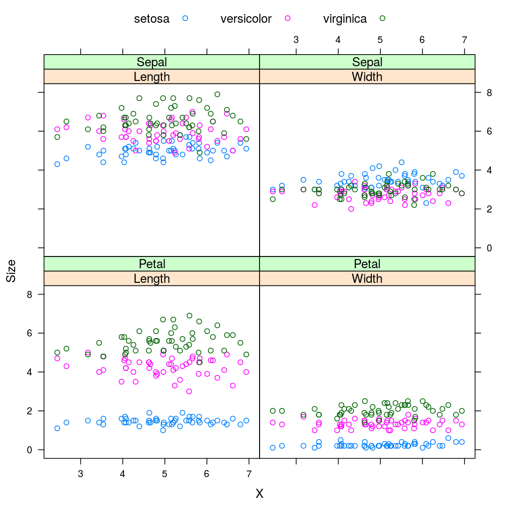
Using iris.D.F (“reverse” sequence) yields

xyplot(Size ~ X | Direction * Floral.Part, data = iris.D.F, groups = Species, auto.key = list(columns = 3))

The two plots are identical since the differences between iris.F.D and iris.D.F—or equivalently between the corresponding sequences of reshapes—are immaterial from the viewpoint of xyplot, as discussed earlier.

How to call reshape and why so?

The crucial but poorly documented feature of reshape is how “time”-varying variables must be specified for the varying argument in factorial experiments like the Iris study. Suppose there are $k$ factors $a_1,...,a_k$, whose levels count $p_{a_1},...,p_{a_k}$ (as we saw these factors are equivalent to index sets $\mathcal{V}_{a_1},...,\mathcal{V}_{a_k}$). With the notation we introduced for longitudinal setups $\prod_{i=1}^k p_{a_1} = p\le n$ because these $k$ factors are fully crossed. The remaining $q\equiv n - p$ variables, if any, are not crossed with the previous $k$ factors and consequently play a passive role in any of the reshapes. In our extended Iris example $p_\mathrm{sp} = 3, \; p_\mathrm{fp} = 2, \; p_\mathrm{dir} = 2$ and $q=1$ because there is a single uncrossed variable: covariate $X$.

To illustrate the sequential use of reshape we will

1. reshape our extended iris into a completely wide format iris.wide
2. then we will reshape iris.wide according to species to obtain iris.2
3. we will check if iris.2 is any different from iris (it should not be apart from implementation details)
4. discuss the semantics behind the syntax of calling reshape

Reshape iris to a completely wide format

It will be convenient to assign the value of the varying argument to reshape to a name, say varying.v.

(varying.v <-
    lapply(c(paste0(".Sepal", c(".Length", ".Width")),
             paste0(".Petal", c(".Length", ".Width"))),
           function(x) paste0(c("Setosa", "Versicolor", "Virginica"), x)))

## [[1]]
## [1] "Setosa.Sepal.Length"     "Versicolor.Sepal.Length"
## [3] "Virginica.Sepal.Length" 
## 
## [[2]]
## [1] "Setosa.Sepal.Width"     "Versicolor.Sepal.Width"
## [3] "Virginica.Sepal.Width" 
## 
## [[3]]
## [1] "Setosa.Petal.Length"     "Versicolor.Petal.Length"
## [3] "Virginica.Petal.Length" 
## 
## [[4]]
## [1] "Setosa.Petal.Width"     "Versicolor.Petal.Width"
## [3] "Virginica.Petal.Width"

That varying.v is indeed the correct argument will be shown and discussed shortly.

Additionally, we create an id variable, whose role is to identify all $m$ observations in the sequence $1,...,m$ repeated for all $3$ levels of species.

iris$id <- rep(seq_len(nrow(iris) / 3), 3)

Now, the syntax of the desired reshape is this:

iris.wide <-
    reshape(iris, direction = "wide",
            varying = varying.v,
            v.names = c("Sepal.Length", "Sepal.Width", "Petal.Length", "Petal.Width"),
            timevar = "Species", times = c("setosa", "versicolor", "virginica"),
            idvar = "id")

The structure of the new data format looks as expected

str(iris.wide)

## 'data.frame':	50 obs. of  14 variables:
##  $ X                      : num  5.65 4.62 6.48 4.79 6.14 ...
##  $ id                     : int  1 2 3 4 5 6 7 8 9 10 ...
##  $ Setosa.Sepal.Length    : num  5.1 4.9 4.7 4.6 5 5.4 4.6 5 4.4 4.9 ...
##  $ Setosa.Sepal.Width     : num  3.5 3 3.2 3.1 3.6 3.9 3.4 3.4 2.9 3.1 ...
##  $ Setosa.Petal.Length    : num  1.4 1.4 1.3 1.5 1.4 1.7 1.4 1.5 1.4 1.5 ...
##  $ Setosa.Petal.Width     : num  0.2 0.2 0.2 0.2 0.2 0.4 0.3 0.2 0.2 0.1 ...
##  $ Versicolor.Sepal.Length: num  7 6.4 6.9 5.5 6.5 5.7 6.3 4.9 6.6 5.2 ...
##  $ Versicolor.Sepal.Width : num  3.2 3.2 3.1 2.3 2.8 2.8 3.3 2.4 2.9 2.7 ...
##  $ Versicolor.Petal.Length: num  4.7 4.5 4.9 4 4.6 4.5 4.7 3.3 4.6 3.9 ...
##  $ Versicolor.Petal.Width : num  1.4 1.5 1.5 1.3 1.5 1.3 1.6 1 1.3 1.4 ...
##  $ Virginica.Sepal.Length : num  6.3 5.8 7.1 6.3 6.5 7.6 4.9 7.3 6.7 7.2 ...
##  $ Virginica.Sepal.Width  : num  3.3 2.7 3 2.9 3 3 2.5 2.9 2.5 3.6 ...
##  $ Virginica.Petal.Length : num  6 5.1 5.9 5.6 5.8 6.6 4.5 6.3 5.8 6.1 ...
##  $ Virginica.Petal.Width  : num  2.5 1.9 2.1 1.8 2.2 2.1 1.7 1.8 1.8 2.5 ...
##  - attr(*, "reshapeWide")=List of 5
##   ..$ v.names: chr  "Sepal.Length" "Sepal.Width" "Petal.Length" "Petal.Width"
##   ..$ timevar: chr "Species"
##   ..$ idvar  : chr "id"
##   ..$ times  : Factor w/ 3 levels "setosa","versicolor",..: 1 2 3
##   ..$ varying: chr [1:4, 1:3] "Setosa.Sepal.Length" "Setosa.Sepal.Width" "Setosa.Petal.Length" "Setosa.Petal.Width" ...

Reverse: from iris.wide to iris.2

Next, the reverse reshape operation is carried out. The syntax is conveniently the same as the forward equivalent except for the direction argument, which has now the value "long".

iris.2 <-
    reshape(iris.wide, direction = "long",
            varying = varying.v,
            v.names = c("Sepal.Length", "Sepal.Width", "Petal.Length", "Petal.Width"),
            timevar = "Species", times = c("setosa", "versicolor", "virginica"),
            idvar = "id")

Checking consistency between iris and iris.2

In fact, iris and iris.2 differ in their attributes, the order of their components, and in the fact that Species is a factor in iris but a character vector in iris.2:

str(iris)

## 'data.frame':	150 obs. of  7 variables:
##  $ Sepal.Length: num  5.1 4.9 4.7 4.6 5 5.4 4.6 5 4.4 4.9 ...
##  $ Sepal.Width : num  3.5 3 3.2 3.1 3.6 3.9 3.4 3.4 2.9 3.1 ...
##  $ Petal.Length: num  1.4 1.4 1.3 1.5 1.4 1.7 1.4 1.5 1.4 1.5 ...
##  $ Petal.Width : num  0.2 0.2 0.2 0.2 0.2 0.4 0.3 0.2 0.2 0.1 ...
##  $ Species     : Factor w/ 3 levels "setosa","versicolor",..: 1 1 1 1 1 1 1 1 1 1 ...
##  $ X           : num  5.65 4.62 6.48 4.79 6.14 ...
##  $ id          : int  1 2 3 4 5 6 7 8 9 10 ...

str(iris.2)

## 'data.frame':	150 obs. of  7 variables:
##  $ X           : num  5.65 4.62 6.48 4.79 6.14 ...
##  $ id          : int  1 2 3 4 5 6 7 8 9 10 ...
##  $ Species     : chr  "setosa" "setosa" "setosa" "setosa" ...
##  $ Sepal.Length: num  5.1 4.9 4.7 4.6 5 5.4 4.6 5 4.4 4.9 ...
##  $ Sepal.Width : num  3.5 3 3.2 3.1 3.6 3.9 3.4 3.4 2.9 3.1 ...
##  $ Petal.Length: num  1.4 1.4 1.3 1.5 1.4 1.7 1.4 1.5 1.4 1.5 ...
##  $ Petal.Width : num  0.2 0.2 0.2 0.2 0.2 0.4 0.3 0.2 0.2 0.1 ...
##  - attr(*, "reshapeLong")=List of 4
##   ..$ varying:List of 4
##   .. ..$ : chr  "Setosa.Sepal.Length" "Versicolor.Sepal.Length" "Virginica.Sepal.Length"
##   .. ..$ : chr  "Setosa.Sepal.Width" "Versicolor.Sepal.Width" "Virginica.Sepal.Width"
##   .. ..$ : chr  "Setosa.Petal.Length" "Versicolor.Petal.Length" "Virginica.Petal.Length"
##   .. ..$ : chr  "Setosa.Petal.Width" "Versicolor.Petal.Width" "Virginica.Petal.Width"
##   ..$ v.names: chr  "Sepal.Length" "Sepal.Width" "Petal.Length" "Petal.Width"
##   ..$ idvar  : chr "id"
##   ..$ timevar: chr "Species"

But do they differ in any meaningful way? Reordering iris.2 and converting its Species component into factor shows

iris.2$Species <- as.factor(iris.2$Species)
all.equal(iris, iris.2[names(iris)])

## [1] "Attributes: < Component \"row.names\": Modes: numeric, character >"              
## [2] "Attributes: < Component \"row.names\": target is numeric, current is character >"

Thus, the answer is: iris.2 does not have any meaningful differences from iris, demonstrating the reversibility of reshape operations with the reshape function. This means that we can perform a sequence of three reshapes from iris.wide and reach essentially the same iris.F.D or iris.D.F as we did with two reshapes from iris.

The semantics and syntax of reshape and its varying argument

When our data are in a completely wide format, a sequence of $k$ reshapes must be used to reach the (completely) long format. Clearly, the sequence of reshapes follows a chosen sequence of factors $a_1,...,a_k$.

First we want to reshape according to factor $a_1$ (equivalently index set $\mathcal{V}_{a_1}$. With what arguments should we call reshape? In particular what should be the value of the varying argument? The above examples show that varying must be a list of character vectors each of length $p_{a_1}$ (see e.g. varying.v in the previous section).

This is because all $p_{a_1}$ levels of factor $a_1$ must appear in each vector. The number of such vectors—the length of the list itself—is $p / p_{a_1} = \prod_{i=2}^k p_{a_i}$ because we need to consider all combinations of the remaining $k-1$ factors. In case of varying.v $a_1 = \mathrm{sp}$ and $p_{a_1}=3$ corresponding to $\{\mathrm{setosa},\mathrm{versicolor},\mathrm{virginica}\}$, this is why each component of the list varying.v is a vector of length $3$. On the other hand, $a_2 = \mathrm{fp}$ and $a_3 = \mathrm{dir}$ so $p / p_{a_1} = p_{a_2} p_{a_3} = 4$ because each of floral part and direction has $2$ levels, and this is why the length of varying.v itself is $4$.

In the second reshape $a_1$ plays no more role so it is omitted from varying. Now the list has $p / (p_{a_1} p_{a_2}) = \prod_{i=3}^k p_{a_i}$ vector components and each vector is $p_{a_2}$ long. The sequence continues with $i=3,...,k$.

If we follow this rule then the last, $k$-th, reshape is special in the sense that no more factors remain and hence we arrive at the nonsense product $\prod_{i=k+1}^k p_{a_i}$ (nonsense since it has zero terms). Then varying is a list with a single component, a $p_{a_k}$-length vector. Such a trivial list may be unlisted: replaced by its only component (the $p_{a_k}$-length vector) without any loss of information. Notice how we could write varying = c("Length", "Width") instead of (the also correct) varying = list("Length", "Width") when we reshaped iris.F into iris.F.D!

In fact, this “final” reshape is probably by far the most frequent way in which reshape is called since it was designed for longitudinal experiments where with only $k=1$ “factor” present: time.

The lessons learned

The multiplicity of data representations is not only computationally convenient but also facilitates the clarification and expression of certain semantic relationships between variables. Unlike stack the reshape function allows representation of various experimental design by partitioning variables into related sets and indexing those separately. We only briefly mentioned how longitudinal experiments can be modeled with reshape and how this can be generalized to cases where instead of time points genes or other objects serve as indices to a set of related variables. reshape’s documentation provides details and examples on—mostly non-generalized—longitudinal applications.

In contrast, we examined more deeply how reshape is also capable of dealing with the equally important but more complex case of factorial experiments, where $k$ number of combined index sets correspond to $k$ crossed factors. In the Iris data set the factors are species, floral part, and measurement direction so $k=3$. Moreover, we supplemented iris with a covariate $X$ with the intention of $X$ having a relation to the original variables akin to time-invariant variables relate time-varying ones in longitudinal studies in a sense that data reshaping is only governed by the latter. This demonstrated how flexibly reshape can be adapted to various setups.

We also saw that as many reshapes can be performed as many factors are present. Therefore various sequences of reshapes may transform a completely wide-format data frame to a completely long-format one. Thus, intermediate formats exist whenever we have $k>2$ factors. Which sequence of reshapes we chose is immaterial, or at least should be, from the viewpoint of well-designed software such as the trellis display plotting xyplot.