1. general task: evaluate arbitrary elements of a sequence of expressions
2. specific task: produce normal Q–Q plots for a sequence of distributions
3. two implementation strategies are discussed: one based on switch and another on substitute
4. using substitute demands more abstract programming but affords more flexibility

A toy problem: recognizing distributions

This exercise appeared in the practicals for chapter 2 of A.C. Davison’s Statistical Models (Cambridge University Press, 2003).

Suppose we want to compare a sequence of distributions to the standard normal distribution. We base the comparison on random samples from the distributions, which we visualize with normal quantile-quantile (Q–Q) plots. For instance, consider the Q–Q plots in the figure titled “Four distributions” below.

To put a twist on this toy problem the sequence $x$ of distributions may contain repeated elements, such as $x = \{\mathrm{gamma}(p), \mathrm{normal}(\mu = 0, \sigma^2 = 1), \mathrm{gamma}(p), \mathrm{gamma}(p)\}$, where $p$ is a vector of parameters for the gamma distribution family. This might be useful if we want to create the following quiz:

1. teacher: generates a sample from each distribution in the sequence $x$ with possibly repeated distributions
   • she/he will sample using either the sample.d.switch or the sample.d.substitute implementation
2. student: creates Q–Q plots from the sequence of samples and guesses $x$, the sequence of distributions
   • she/he will plot the samples using plot.ls

To keep things simple, we will sample the same number of points $n$ from each distribution and for the parameters of all distributions will be based on a single number $m$ with the constraint that all distributions should be on comparable scale so that the principal difference is in the shape of the distributions. We store $n$ and $m$ in the list param.

param <- list(n = 100, m = 5)

The student’s Q–Q plotting function

The plot.ls function defined below uses qqmath of the lattice package to produce a trellis plot, where each panel is the normal Q–Q plot of one sample from the sequence of samples s. Our plot.ls expects s to be implemented as an unnamed list of named lists. Each named list has an element named family that specifies the family of the distribution, an element named sample that contains the sample points, and an element named i that specifies the index of the distribution in the sequence.

If guess argument is FALSE, then plot.ls will display the name of the distribution family on the top of each panel. Otherwise the student must guess the families. In the latter case she/he can check the answers by printing the return value of plot.ls. A few more details on plot.ls will be given later.

plot.ls <- function(s, guess = FALSE, call2strip = FALSE, ...) {
    dt <- do.call(rbind, lapply(s, data.frame))
    d.names <- sapply(s, getElement, "family")
    tp <-
        qqmath(~ sample | i, data = dt,
               strip = strip.custom(factor.levels = d.names),
               strip.left =
                   if(call2strip)
                       strip.custom(factor.levels = sapply(s, getElement, "call"), par.strip.text = list(cex = 0.65))
                   else FALSE,
                   xlab = "normal quantiles", ylab = "sample quantiles", as.table = TRUE, between = list(x = 1, y = 1),
                   abline = c(0, 1), pch = "+",
                   ...)
    if(guess) tp <- update(tp, strip = strip.custom(factor.levels = as.character(seq_along(s))),
                           strip.left = FALSE, main = "Guessing distributions")
    print(tp)
    if(guess) d.names
}

The teacher’s sampling function using “switch”

sample.d.switch specifies four distributions. Each distribution is represented as a named list with the family, sample and i components mentioned above. The unnamed list of these named lists appears the (unnamed) list of “alternatives” passed switch in the body of sample.d.switch. The arguments of sample.d.switch itself are x and p. The x argument is a sequence of possibly repeated indices of arbitrary length; each index selects one of the four distributions specified within switch therefore must range between 1 and 4. The p argument contains information on sample sizes and parameter values, and defaults to the param list defined above.

sample.d.switch <- function(x = 1:4, p = param) {
    n <- p$n
    m <- p$m
    helper <- function(i) {
        switch(x[i],
               list(family = "normal", sample = rnorm(n), i = factor(i)),
               list(family = "t", sample = rt(n, df=m), i = factor(i)),
               list(family = "gamma", sample = rgamma(n, shape=m) / m, i = factor(i)),
               list(family = "rounded.normal", sample = round(m * rnorm(n)) / m, i = factor(i)))
    }
    lapply(seq_along(x), helper)
}

Let’s see how the teacher generates a sequence s of samples using sample.d.switch! She/he decides to pass the default x = 1:4 argument, which results in the original sequence of four unique (not repeated) distributions.

set.seed(1993) # the year R appeared
str(s <- sample.d.switch(x = 1:4))

## List of 4
##  $ :List of 3
##   ..$ family: chr "normal"
##   ..$ sample: num [1:100] -0.5005 -0.3772 0.0435 -0.6507 1.1533 ...
##   ..$ i     : Factor w/ 1 level "1": 1
##  $ :List of 3
##   ..$ family: chr "t"
##   ..$ sample: num [1:100] -1.074 1.623 -0.817 0.934 -0.133 ...
##   ..$ i     : Factor w/ 1 level "2": 1
##  $ :List of 3
##   ..$ family: chr "gamma"
##   ..$ sample: num [1:100] 0.47 0.819 0.98 0.566 1.206 ...
##   ..$ i     : Factor w/ 1 level "3": 1
##  $ :List of 3
##   ..$ family: chr "rounded.normal"
##   ..$ sample: num [1:100] 0.4 0.2 -0.8 0.6 1.8 0.6 0 -0.2 0 0.6 ...
##   ..$ i     : Factor w/ 1 level "4": 1

The teacher tells the student to first plot the sequence of samples with plot.ls and display the families as well so that the student can analyze their shapes before having to solve the “real” exercise: the reverse task, that is.

library(lattice)
plot.ls(s = s, guess = FALSE, main = "Four distributions")

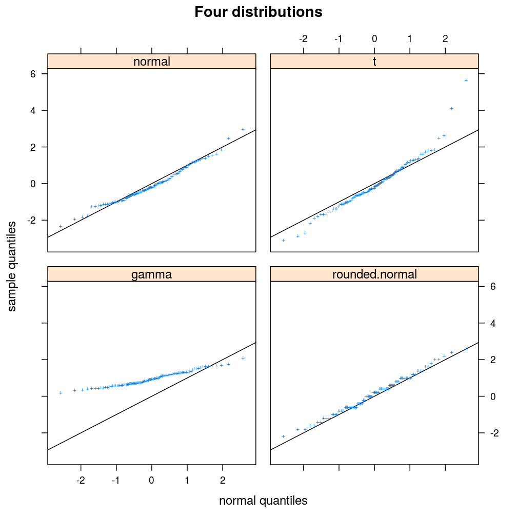
The student notes that, relative to the standard normal distribution, the t distribution has heavier tails, the gamma distribution is not supported on negative numbers, and that the effect of rounding is a step-like pattern in the Q–Q plot.

Now the teacher challenges the student with a sequence of six samples, three of which (#2, #3, #5) are from the t distribution, two (#4, #6) from the normal distribution and one (#1) from the gamma.

s <- sample.d.switch(x = c(3, 2, 2, 1, 2, 1))

When the student plots these samples with guess = TRUE, this is what she/he sees:

library(lattice)
ans <- plot.ls(s = s, guess = TRUE)

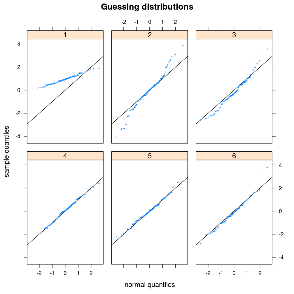
Once she/he guessed the distributions, the correct answers are printed.

ans

## [1] "gamma"  "t"      "t"      "normal" "t"      "normal"

The teacher’s sampling function using “substitute”

The teacher is dissatisfied by two limitations of sample.d.switch.

Firstly, it would be important for the student to understand the role of parameters in the shape of various distributions, and also to get accustomed to the syntax of the R functions in the stats package. In fact, the student wrote plot.ls with these considerations in mind when she/he included an argument named call2strip. If call2strip = TRUE, then plot.ls displays on the right side of each panel the expression with which a function like rgamma was called in sample.d.switch. However, the return value of sample.d.switch contains no information on those function calls.

The second limitation is the lack of modularity that follows from the fact that the set of four distinct distributions are tied to the body of sample.d.switch. How can more distinct distributions be added to the exercise without changing the body of the sampling function?

The second limitation might be overcome by somehow passing the list of “alternatives”, say ld, to the main sampling function that would then call switch with ld as arguments. But that strategy would have to be involve do.call as well as the prepending of ld with an index that selects a single element from it. But the first limitation can be overcome in a straight-forward way only by using substitute.

So, the teacher implements sample.d.substitute. The x and p arguments have the same semantics as in the case of sample.d.switch. The new argument is ld, the unnamed list of named lists.

sample.d.substitute <- function(x = 1:4, ld, p = param) {
    helper <- function(i) {
        le <- list(e = ld[[x[i]]])
        cl <- eval(substitute(substitute(e, p), le))
        list(family = names(ld[x[i]])[[1]],
             call = deparse(cl),
             sample = eval(cl),
             i = factor(i))
    }
    lapply(seq_along(x), helper)
}

Now the set of four distinct distributions can be stored in a l.distr, a list of lists, which exists separately from sample.d.substitute.

l.distr <- list(normal = quote(rnorm(n = n)),
                t = quote(rt(n = n, df = m)),
                gamma = quote(rgamma(n = n, shape = m) / m),
                rounded.normal = quote(round(m * rnorm(n = n)) / m))

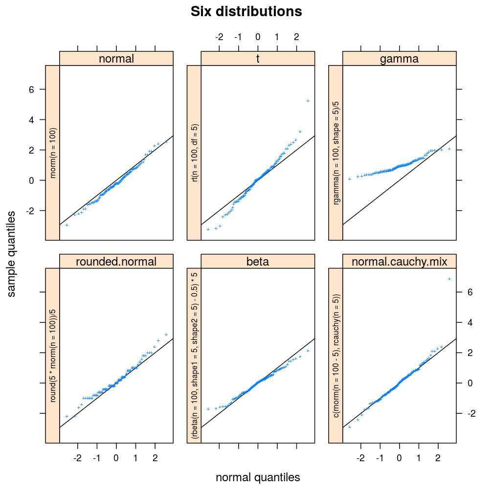
But before the teacher tests sample.d.substitute she/he decides to add two more distinct distributions to l.distr.

# extend list of distributions
l.distr$beta <- quote((rbeta(n = n, shape1 = m, shape2 = m) - 0.5) * m)
l.distr$normal.cauchy.mix <- quote(c(rnorm(n = n - m), rcauchy(n = m)))

Now, the system is ready for the test.

s <- sample.d.substitute(x = 1:6, ld = l.distr)
plot.ls(s = s, guess = FALSE, call2strip = TRUE, main = "Six distributions")

The teacher likes sample.d.substitute so much that she/he starts exercising with it.

set.seed(13) # challenging superstition
s <- sample.d.substitute(sample(seq_along(l.distr), 10, replace = TRUE), ld = l.distr)
ans <- plot.ls(s = s, guess = TRUE, layout = c(5, 2))

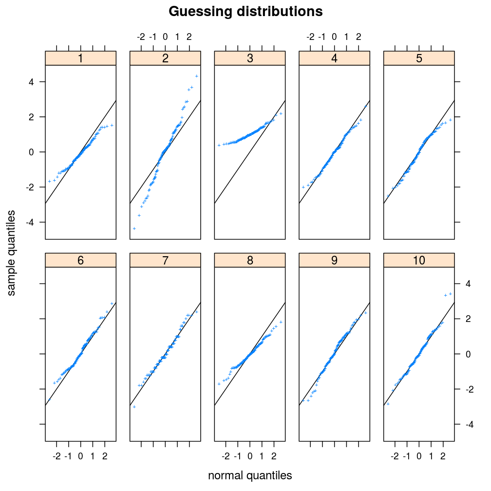
Checking answers:

ans

##  [1] "beta"              "t"                 "gamma"            
##  [4] "normal"            "normal.cauchy.mix" "normal"           
##  [7] "rounded.normal"    "beta"              "normal.cauchy.mix"
## [10] "normal"

Why substitution works better

Clearly, the new implementation based on sample.d.substitute and a separate input list overcame the limitations of sample.d.substitute. What made that possible?

Comparing the code for sample.d.substitute with that of sample.d.switch shows, that the main change was the replacement of the switch expression by several expressions that involve two calls to substitute and two calls to eval. Let’s look at the most relevant part of the code of sample.d.substitute!

1   sample.d.substitute <- function(x = 1:4, ld, p = param) {
2       ....
3           le <- list(e = ld[[x[i]]])
4           cl <- eval(substitute(substitute(e, p), le))
5           ....
6                call = deparse(cl),
7                sample = eval(cl),
                 ....
        ....

Note that argument ld in line 1 is a list of quoted (that is: unevaluated) expressions like rnorm(n = n). In line 3 a single expression is selected from ld using the index x[i] and that expression is named e within the named list le. So, if x[i] takes the value of 1 then e is rnorm(n = n) while if x[i] is, say, 6 then e is c(rnorm(n = n - m), rcauchy(n = m)).

Line 4 evaluates substitute(substitute(e, p), le) in multiple steps. First, the outer substitute replaces e by the value of le$e, which is the unevaluated expression c(rnorm(n = n - m), rcauchy(n = m)) if we select the 6th element of l.distr. We assign the value of the first substitute to s1 so that we can print it:

# p and le in the workspace instead of the body of sample.d.substitute 
p <- list(n = 77, m = 4)
le <- list(e = l.distr[[6]])
(s1 <- substitute(substitute(e, p), le))

## substitute(c(rnorm(n = n - m), rcauchy(n = m)), p)

Now the second substitution takes place that replaces the second n in the argument list of rnorm with the value of n in the named list list(n = 77, m = 4), which is 77. It does not replace the first n symbol in rnorm neither the only n symbol in rcauchy because both of those instances of the n symbol stand for the name of these functions’ sample size argument (in scheme they are called formal parameters). Such complication does not arise with m because that symbol identifies no argument name in rnorm or rcauchy, so both instances of m are replaced with 4. But the second substitution cannot occur without eval because substitute(c(rnorm(n = n - m), rcauchy(n = m)), p), the value of s1, is an unevaluated expression just like rnorm(n = n) and the others in l.distr. In this sense it does not matter that the value of s1 happens to contain the symbol substitute while rnorm(n = n) does not; both expressions are unevaluated until passed to eval. When this happens to s1, only then does it gain significance that s1 names an expression that begins with substitute. Evaluation of such expression results in a new unevaluated expression with all the replacements, concerning symbols in p, having taken place.

(cl <- eval(s1))

## c(rnorm(n = 77 - 4), rcauchy(n = 4))

This expression is specific both to the index of l.distr, in this case 6, and to the value of p, in this case list(n = 77, m = 4). The two substitutions were necessary to isolate the specification of the family of the distribution from the specification of its parameters.

Now we can do two things with the unevaluated expression cl, which is formally a call object. First, as in line 6 above, we can deparse it into a character vector to use it in various figure labels.

deparse(cl)

## [1] "c(rnorm(n = 77 - 4), rcauchy(n = 4))"

Second, as in line 7 above, we can evaluate it to generate the statistical sample, implemented as a numeric vector.

str(eval(cl))

##  num [1:77] -0.621 -0.214 -0.506 0.93 -0.913 ...

cl is used in both ways in sample.d.substitute and that is one of the reasons why that function is superior to sample.d.switch. The other reason is the modularity enabled by the passing of unevaluated expressions (e.g. rnorm(n = n)) to sample.d.substitute. The cost of this implementation is having to deal with the non-standard way of evaluation, which is more difficult to analyze and debug for most programmers who are already well accustomed to the standard evaluation in R.