Fixed and Mixed Regression Models

Fixed and mixed models are fitted to the sleepstudy dataset to investigate how human reaction slows down with sleep deprivation.

Sleep study

A sleep study was carried out to investigate whether and how reaction time slows down with sleep deprivation. The corresponding sleepstudy dataset is part of the lme4 package; below is the description of sleepstudy:

The average reaction time per day for subjects in a sleep deprivation study. On day 0 the subjects had their normal amount of sleep. Starting that night they were restricted to 3 hours of sleep per night. The observations represent the average reaction time on a series of tests given each day to each subject.

This data set is ideal to compare fixed and mixed effects models. The outline of this article is as follows:

inspect the data
mathematical description and fitting of models
1. F1, a fixed effects model
2. M1 and M2, two mixed models
fitting the models
statistical inference (using F1, M1, M2)

Inspecting the data

First some prerequisites…

library(lme4)

## Loading required package: Matrix

## Loading required package: methods

library(lattice)
lattice.options(default.args = list(as.table = TRUE))
lattice.options(default.theme = "standard.theme")
opts_chunk$set(dpi = 144)
opts_chunk$set(fig.width = 6)
opts_chunk$set(fig.asp = 1)
opts_chunk$set(out.width = "700px")
opts_chunk$set(dev = c("png", "pdf"))
tp <- list(superpose.line = list(col = c("black", "orange", "red", "brown", "green4", "blue", trellis.par.get("superpose.line")$col[-1:-5])))
tp$superpose.symbol <- tp$superpose.line
tp$plot.symbol <- tp$plot.symbol <- list(col = tp$superpose.line$col[1])
source("2017-10-16-fixed-and-mixed-models.R")

The human subjects of sleepstudy are numbered in a way that’s a little inconvenient for our purposes, so let’s simplify and renumber them from 1 to 18 and look at the first 3 and last 3 data points!

sleepstudy <- sleepstudy
levels(sleepstudy$Subject) <- seq_along(levels(sleepstudy$Subject))
rbind(head(sleepstudy, 3), tail(sleepstudy, 3))

##     Reaction Days Subject
## 1   249.5600    0       1
## 2   258.7047    1       1
## 3   250.8006    2       1
## 178 343.2199    7      18
## 179 369.1417    8      18
## 180 364.1236    9      18

Now let’s plot the average reaction time against the test day for each subject!

xyplot(Reaction ~ Days | Subject, data = sleepstudy, layout = c(6, 3), par.settings = tp, auto.key = list(text = "sleep study", points = FALSE), ylim = c(175, 485))

plot of chunk data

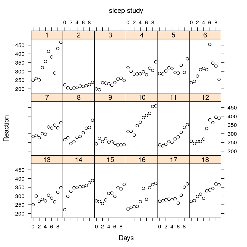
The plot shows that subjects vary with respect to…

their initial reaction time (at day 0)
how their reaction time changes systematically with days
how scattered the data points are (noise, non-systematic variation)

But the plot also reveals common patterns shared by the subjects: for most of them the reaction time is initially $\approx 250$ milliseconds but this value tends to rise systematically with days suggesting that sleep deprivation slows down reaction.

We seek models that are able to capture as much of the varying and shared patterns noted above as possible. We’ll evaluate that ability in terms of how well each model fits the data. Then we will use the models to test if the dependence of reaction time indeed varies across subjects and whether in a typical or average subject that dependence is indeed positive, as the scatter plot above suggests.

Mathematical description of models

Before plunging into model descriptions it helps to make some considerations about notation. We’ll index the 18 subjects with $g=1,...,G=18$ . Observations are indexed with $i$ . Data points for the reaction time (the response variable) and days of sleep deprivation (the explanatory variable) are denoted as $y_{gi}$ and $x_{gi}$ , respectively. The noise is denoted as $\varepsilon_{gi}$ . Any other Greek letter ( $\beta, \gamma, \delta, \alpha$ ) will denote regression coefficients.

F1, a fixed effects model

This is the familiar normal linear model for each subject $g$ .

$\begin{eqnarray*} y_{gi} &=& \alpha_g + x_i \beta_g + \varepsilon_{gi} \\\\ \varepsilon_{gi} &\sim& \mathcal{N}(0, \sigma_g^2). \end{eqnarray*}$

Thus $F1$ is a set of such models that are isolated from each other in the sense that they share no parameters or data.

In hypothesis testing we’ll make use of a “null model” $F0$ , which is a constrained version of $F1$ by asserting that

$\begin{equation} F0: \; \beta_g = 0 \end{equation}$

Thus, $F0$ assumes independence between reaction time and days of sleep deprivation.

M1 and M2, two mixed models

We consider two mixed models that allow dependence of reaction time on days of sleep deprivation, $M1$ and $M2$ . In addition, we’ll make use of a third mixed model, a “null model” $M0$ , in which reaction time is independent of days. These are nested: $M2 \supset M1 \supset M0$ , meaning that $M1$ and $M0$ can be derived from $M2$ by constraining certain parameters. Although both $M1$ and $M2$ account for the increasing tendency of reaction time with days (while $M0$ does not), only $M2$ allows subjects to vary with respect to how reaction time depends on days. All 3 models $M0, M1, M2$ allow the average reaction time to vary across subjects.

After the above qualitative description we specify the models qualitatively. Both models share the following form and properties:

$\begin{eqnarray*} y_{gi} &=& \alpha + a_g + x_i (\beta + b_g) + \varepsilon_{gi} \\\\ a \equiv (a_1, ..., a_G) &\sim& \mathcal{N}(0, \Omega_a) \\\\ \varepsilon_{gi} &\sim& \mathcal{N}(0, \sigma^2). \end{eqnarray*}$

In addition, $\beta$ is an unknown fixed parameter both in $M1$ and $M2$ .

The only difference between $M1$ and $M2$ is $b \equiv (b_1, ..., b_G)$ ; in $M2$ it is allowed to vary randomly while in $M1$ it is constrained to be 0. $M0$ differs from $M1$ in that $\beta$ is constrained to zero. $\begin{eqnarray*} M2: \; b &\sim& \mathcal{N}(0, \Omega_b) \\\\ M1: \; b &=& 0 \\\\ M0: \; b &=& 0, \; \beta = 0 \end{eqnarray*}$

Fitting the models

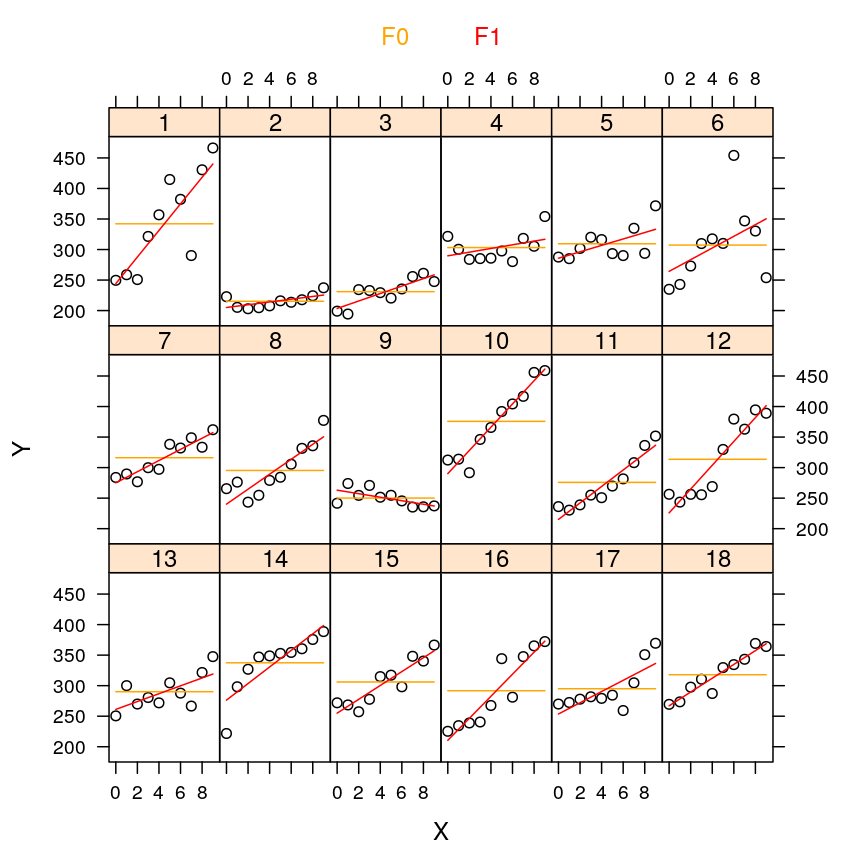
The stats package provides the lm function for fitting (normal, linear) fixed effects models. Our fixed model F1 is the set of all such (sub)models, each fitted to a different subject.

subjects <- levels(sleepstudy$Subject)
names(subjects) <- subjects
M <- list()
M$F0 <-
    lapply(subjects,
           function(s) {
               df <- subset(sleepstudy, Subject == s)
               lm(Reaction ~ 1, data = df)
           })
M$F1 <-
    lapply(subjects,
           function(s) {
               df <- subset(sleepstudy, Subject == s)
               lm(Reaction ~ Days, data = df)
           })

M$M0 <- lmer(Reaction ~ (1 | Subject), sleepstudy)
M$M1 <- lmer(Reaction ~ Days + (1 | Subject), sleepstudy)
M$M2 <- lmer(Reaction ~ Days + (Days | Subject), sleepstudy)

df <- cbind(sleepstudy,
            data.frame(yhat.F0 = unlist(lapply(M$F0, predict)),
                       yhat.F1 = unlist(lapply(M$F1, predict)),
                       yhat.M0 = predict(M$M0),
                       yhat.M1 = predict(M$M1),
                       yhat.M2 = predict(M$M2)))
names(df) <- sub("Days", "X", names(df))
df.long <- reshape(df, varying = varying <- c("Reaction", "yhat.F0", "yhat.F1", "yhat.M0", "yhat.M1", "yhat.M2"), v.names = "Y", timevar = "Type", direction = "long", times = varying)
df.long$Type <- factor(df.long$Type)
levels(df.long$Type) <- c("data", "F0", "F1", "M0", "M1", "M2")

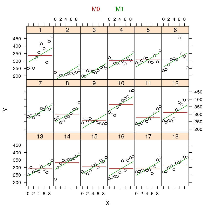
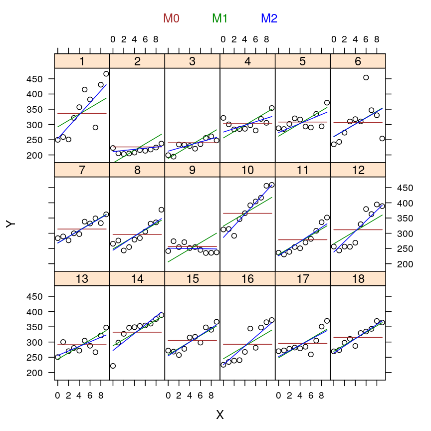
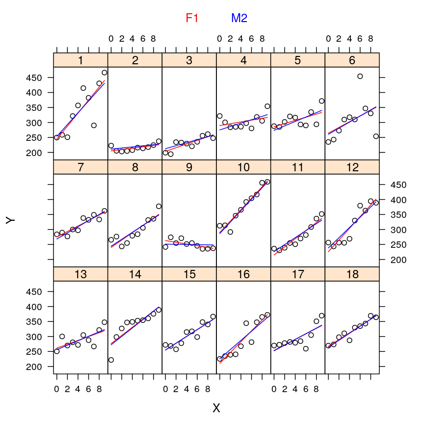
The TODO lines represent the fitted line under M2, the TODO lines under M1 (the observed data remain cyan).

my.xyplot <- function (selection = c(2,3), dframe = df.long, tpar = tp)
    xyplot(Y ~ X | Subject, data = dframe, groups = Type, type = c("p", rep("l", 5)), subset = Type %in% levels(Type)[c(1, selection)], distribute.type = TRUE, par.settings = tpar, auto.key = list(text = levels(dframe$Type)[selection], points = FALSE, lines = FALSE, columns = length(selection), col = tpar$superpose.line$col[selection]), layout = c(6, 3), ylim = c(175, 485))
my.xyplot(c(2,3))

plot of chunk data-F0-F1

my.xyplot(c(4:5))

plot of chunk data-M0-M1

my.xyplot(c(4:6))

plot of chunk data-M0-M1-M2

my.xyplot(c(3, 6))

plot of chunk data-F1-M2

Statistical inference using fixed and mixed models

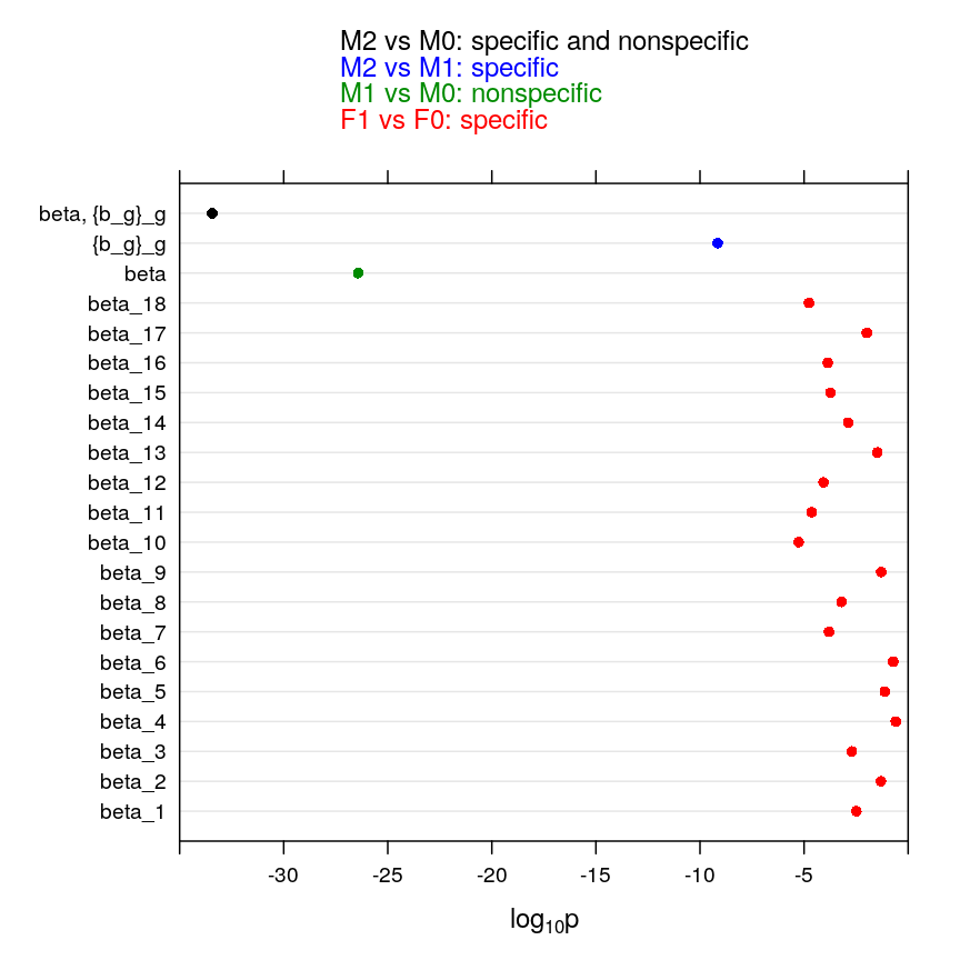
Several hypotheses appear relevant for sleepstudy: that reaction time and sleep deprivation are independent, that they are dependent invariably across subjects, or that the dependence varies across subjects. Mathematically, a null hypothesis is a constraint on a parameter. We will focus on the slope parameters of various models whether they mediate fixed effects ( $\{\beta_g\}_{g=1,...G}, \beta$ ) or random effects( $\{b_g\}_{g=1,...,G}$ ). Thus to each null hypothesis corresponds a “null” model in which some of the slope parameters are constrained to zero. This null model will be compared to a more general (less constrained) alternative model. Note that the same model may play the role of both a null or an alternative model depending on which hypothesis we test. Also recall that the most powerful test when the null model is nested in the alternative one is the likelihood ratio test. The likelihood ratio test is known as ANOVA for the special case of regression models, such as ours.

H <- list()
H$pval <- sapply(names(M$F1), function(x) anova(M$F0[[x]], M$F1[[x]])[2, "Pr(>F)"])
# alternative method, which gives same result
all.equal(H$pval,
          sapply(M$F1, function(m) summary(m)$coefficients["Days", "Pr(>|t|)"]))

## [1] TRUE

H$col <- tp$superpose.line$col[3]
H$ANOVA <- "F1 vs F0"
H <- data.frame(H)
H$par <- paste0("beta_", seq_along(H$pval))
H$H0 <- paste0("beta_", seq_along(H$pval), " = 0")

H <- rbind(H,
           data.frame(pval = anova(M$M0, M$M1)[2, "Pr(>Chisq)"],
                      col = tp$superpose.line$col[5],
                      ANOVA = "M1 vs M0",
                      par = "beta",
                      H0 = "beta = 0"),
           data.frame(pval = anova(M$M1, M$M2)[2, "Pr(>Chisq)"],
                      col = tp$superpose.line$col[6],
                      ANOVA = "M2 vs M1",
                      par = "{b_g}_g",
                      H0 = "{b_g = 0}_g"),
           data.frame(pval = anova(M$M0, M$M2)[2, "Pr(>Chisq)"],
                      col = tp$superpose.line$col[6],
                      ANOVA = "M2 vs M0",
                      par = "beta, {b_g}_g",
                      H0 = "beta = 0, {b_g = 0}_g")
           )

## refitting model(s) with ML (instead of REML)
## refitting model(s) with ML (instead of REML)
## refitting model(s) with ML (instead of REML)

H$par <- factor(H$par, levels = H$par, ordered = TRUE)
H$H0 <- factor(H$H0, levels = H$H0, ordered = TRUE)

my.dotplot <- function(dt = H, select = c("F1 vs F0", "M1 vs M0", "M2 vs M1", "M2 vs M0"), ...) {
    sel <- dt$ANOVA %in% select
    ssel <- levels(dt$ANOVA) %in% select
    txt <- rev(c("F1 vs F0: specific", "M1 vs M0: nonspecific", "M2 vs M1: specific", "M2 vs M0: specific and nonspecific"))
    dotplot(par ~ log10(pval), data = dt, subset = sel,
            auto.key = list(text = ifelse(rev(ssel), txt, ""),
                            col = rev(c("red", "green4", "blue", "black")), points = FALSE),
            xlab = expression(paste(log[10], "p")),
            scales = list(y = list(limits = c(0, nrow(dt) + 1), at = seq_len(nrow(dt)), labels = dt$par)),
            xlim = c(-35, 0),
            par.settings = list(dot.symbol = list(col = c(as.character(dt$col)[-length(dt$col)], "black"))),
            ...)
}

my.dotplot()

plot of chunk unnamed-chunk-8

pdf(file = "figure/p-val-F1F0.pdf")
my.dotplot(select = c("F1 vs F0"))
dev.off()
pdf(file = "figure/p-val-F1F0-M1M0.pdf")
my.dotplot(select = c("F1 vs F0", "M1 vs M0"))
dev.off()
pdf(file = "figure/p-val-F1F0-M1M0-M2M1-M2M0.pdf")
my.dotplot(select = c("F1 vs F0", "M1 vs M0", "M2 vs M1", "M2 vs M0"))
dev.off()

Implications to our study

Mixed models would afford joint modeling of the data across all 30 genes in a way that the effect of each predictor (e.g. Age) could possibly be divided into a global component (a fixed effect shared by all genes) and a gene-specific component (a gene-specific random effect). Compared to the previous strategy of separate gene-specific models the proposed joint modeling would extend the formally testable hypotheses to those that involve all genes jointly. Thus the main advantages would be

increased power of currently unresolved hypotheses e.g. the overall effect of Age taking all genes into account
more hypotheses may be tested by separating gene-specific effects from effects shared by all genes

Note that the increased power follows from the fact that joint modeling allows borrowing of strength from data across all genes and that powerful likelihood ratio tests could be easily formulated by comparing nested models. Additional benefits:

better separation of technical and biological effects
- for instance, we could model Institution-specific effect of RIN or RNA_batch and gene-specific effect of Age, Dx, or Ancestry.1
shrinkage: for genes with many observations let the data “speak for themselves” but for data-poor genes shrink gene-specific parameters to a global average
more straight-forward model comparison
- various model families and data transformations
- nested models (likelihood ratio tests)