Decision tree model is fitted to toy data on homes in New York and San Francisco (NY, SF). Along the way overfitting is illustrated. The optimally fitted tree is used to classify some test data as either NY or SF.
Download the related presentation here
Data and analytical tools
We are going to use the home data and the machine learning approach called decision tree or CART (Classification And Regression Tree) from A visual introduction to machine learning, referred to here as visual intro. As CART implementation we are going to take advantage of the rpart package. As usual in this blog, we opt for lattice graphics.
library(lattice)
library(rpart)
lattice.options(default.args = list(as.table = TRUE))
lattice.options(default.theme = "standard.theme")
opts_chunk$set(dpi = 144)
opts_chunk$set(out.width = "700px")
opts_chunk$set(dev = c("png", "pdf"))
Now read the data…
home <- read.csv("ny-sf-home-data.csv")
home <- cbind(data.frame(city = factor(home$in_sf)), home)
levels(home$city) <- c("NY", "SF")
head(home, n = 2)
##   city in_sf beds bath   price year_built sqft price_per_sqft elevation
## 1   NY     0    2    1  999000       1960 1000            999        10
## 2   NY     0    2    2 2750000       2006 1418           1939         0
tail(home, n = 2)
##     city in_sf beds bath  price year_built sqft price_per_sqft elevation
## 491   SF     1    1    1 649000       1983  850            764       163
## 492   SF     1    3    2 995000       1956 1305            762       216
So our data are 492 observations on homes in two cities: New York and San Francisco (). We’ll treat (equivalent to the variable) as a categorical output with classes . The rest of variables (except for ) will be treated as input.
Here we reproduce the scatter plot matrix from visual intro.
trellis.par.set(superpose.symbol = list(pch = 20, alpha = 0.2, col = c(my.col <- c("blue", "green3"), trellis.par.get("superpose.symbol")$col[3:7])))
splom(~ home[3:9], data = home, groups = city, auto.key = TRUE, pscales = 0)

Elevation seems like an input variable that is informative for distinguishing NY from SF. But the empirical distribution of elevation for NY overlaps considerably with SF at lower elevations. Therefore additional variables like would be useful for training a good classifier.
densityplot(~ elevation | city, data = home, groups = city, plot.points = "rug", layout = c(1, 2), xlim = c(0, 250), col = my.col)

xyplot(elevation ~ price_per_sqft, data = home, groups = city, col = my.col, auto.key = TRUE)

CART / decision tree
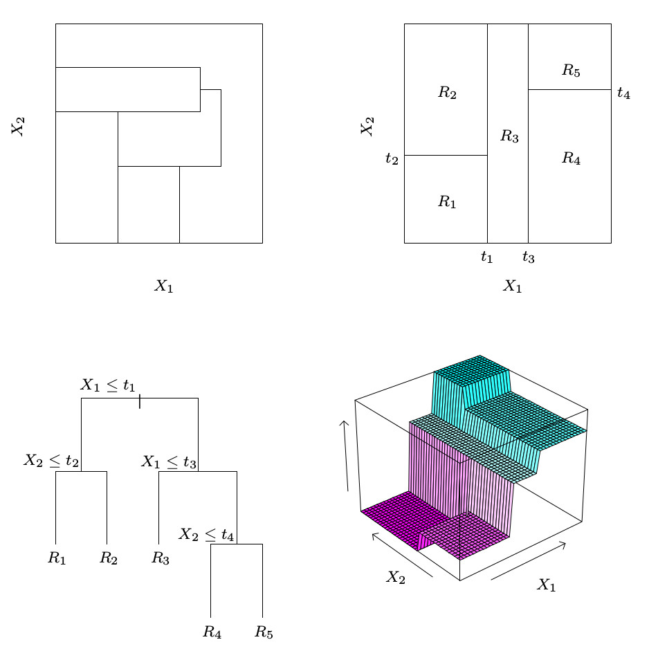
This figure 9.2 from Hastie et al 2009 explains the recursive partitioning of CART. Visual intro provides elegant dynamic visualization of the fitting process.
We first fit the decision tree with control = rpart.control(cp = -1), which allows the tree to grow beyond optimal size and thus overfit the data.
M <- list()
M$complex.tree <- rpart(city ~ beds + bath + price + year_built + sqft + price_per_sqft + elevation, data = home, control = rpart.control(cp = -1))
plot(M$complex.tree, margin = 0.01)
text(M$complex.tree, col = "brown", font = 2, use.n = FALSE, all = FALSE, cex = 0.8)

The table and plot show the complexity parameter table at 7 different “prunings” sequentially nested in the overfitted tree above. 8 splits correspond to the optimal pruning.
printcp(M$complex.tree)
##
## Classification tree:
## rpart(formula = city ~ beds + bath + price + year_built + sqft +
##     price_per_sqft + elevation, data = home, control = rpart.control(cp = -1))
##
## Variables actually used in tree construction:
## [1] bath           elevation      price          price_per_sqft
## [5] sqft           year_built
##
## Root node error: 224/492 = 0.45528
##
## n= 492
##
##           CP nsplit rel error  xerror     xstd
## 1  0.5803571      0   1.00000 1.00000 0.049313
## 2  0.0892857      1   0.41964 0.43304 0.039396
## 3  0.0267857      3   0.24107 0.26786 0.032403
## 4  0.0089286      5   0.18750 0.27232 0.032634
## 5  0.0066964      6   0.17857 0.25446 0.031692
## 6  0.0000000      8   0.16518 0.25000 0.031449
## 7 -1.0000000     17   0.16518 0.25000 0.031449
plotcp(M$complex.tree, upper = "splits")

Thus the optimal tree is the one below and this model will be used for the classification tasks in the next section. Notice how only a subset of input variables appear on the tree so that the rest are deemed uninformative. Moreover, and each appear at two splits, which underscores their importance.
M$tree <- rpart(city ~ beds + bath + price + year_built + sqft + price_per_sqft + elevation, data = home)
plot(M$tree, margin = 0.01)
text(M$tree, col = "brown", font = 2, use.n = TRUE, all = TRUE, cex = 0.9)

Classification
Let’s predict the city at the average of each input variable taking the following values:
(newhome <- data.frame(lapply(home[c(-1, -2)], function(h) round(mean(h)))))
##   beds bath   price year_built sqft price_per_sqft elevation
## 1    2    2 2020696       1959 1523           1196        40
Now the prediction. Actually, it’s more than mere prediction of the output classes (NY and SF) because their probability is estimated. Note that the first splitting rule of the tree already classifies the new data point as SF because . Therefore the model based probability estimates are compared to the fraction of those NY and SF homes in the training data whose , which is . The two kinds of probability estimate are only slightly different: they agree that :
nh.prob <- predict(M$tree, newhome, type = "prob")
nh.prob <- rbind(nh.prob, data.frame(NY = 9 / 183, SF = (183 - 9) / 183))
nh.prob$prob.estimate <- c("prediction", "training data, elevation >= 30.5")
nh.prob
##            NY        SF                    prob.estimate
## 1  0.04687500 0.9531250                       prediction
## 11 0.04918033 0.9508197 training data, elevation >= 30.5
nh.prob <- reshape(nh.prob, varying = c("NY", "SF"), v.names = "probability", times = c("NY", "SF"), timevar = "city", direction = "long")
barchart(probability ~ prob.estimate, data = nh.prob, groups = city, stack = TRUE, auto.key = TRUE, scales = list(x = list(cex = 1)))

The next prediction is at a sequence of increasing in the range of the training data, while holding all other input variables at their average.
nh <- cbind(newhome[-6], data.frame(price_per_sqft = seq(from = min(home$price_per_sqft), to = max(home$price_per_sqft), length.out = 50)))
nh.prob <- predict(M$tree, nh, type = "prob")
my.xyplot <- function(fm = formula(NY ~ price_per_sqft), newdata = nh, mod = M)
    xyplot(fm, data = cbind(newdata, predict(mod$tree, newdata, type = "prob")),
           ylim = c(-0.05, 1.05), ylab = "Pr(city = NY)",
           panel = function(...) { panel.grid(h = -1, v = -1); panel.xyplot(...) })
my.xyplot()

Clearly, the model based probability estimates show no dependence on , because the tree ends in a leaf if (the right branch of the first split). So let’s set and repeat the prediction. This time there is a clear dependence on . It is a striking limitation of the decision tree model that the dependence is step-like. Note that the step is located at , which corresponds to the second of the two splits based on . There is a tiny step at corresponding to the first of the splits based on . This tiny step goes counter-intuitively downward exposing another weakness of decision trees.
nh$elevation <- 30
my.xyplot()

Finally, let’s do the same type of experiment when grows incrementally. Similarly to the previous case, there is a sudden jump around a splitting threshold, which is in this case , corresponding to the first (topmost) split in the tree.
nh <- cbind(newhome[-7], data.frame(elevation = seq(from = min(home$elevation), to = max(home$elevation), length.out = 50)))
my.xyplot(fm = formula(NY ~ elevation))
