Previous analysis by Ifat analyzed the relationship between age and allelic imbalance by fitting a normal linear model to rank-transformed values averaged over a set of genes. My follow-up analysis extended this to a set of genes. Here alternative models are fitted directly to the (untransformed) values. Furthermore, all models are fitted to not only aggregated gene sets but also single genes. Models are compared based on the Akaike information criterion (AIC).
Preparations
source('2016-04-22-glm-for-s-statistic.R') # functions for data filtering and fitting
source('2016-04-22-glm-for-s-statistic-run.R') # do filtering and fitting
source('2016-04-22-glm-for-s-statistic-graphs.R') # graphics functions
source('2016-04-22-glm-for-s-statistic-graphs-run.R') # some objects for graphing
source('../2016-03-02-ifats-regression-analysis/2016-03-02-ifats-regression-analysis.R') # Ifat's implementation of fitting
Data
Data files:
files <- list(S="pop_skew_3June15.txt",
              N="pop_cov_3June15.txt",
              X="DLPFC.ensembl.KNOWN_AND_SVA.ADJUST.SAMPLE_COVARIATES.tsv",
              X2="samples.csv")
File S contains the matrix of the observed statistic for all individuals and selected genes . (The capitalized denotes the corresponding random variable). Similarly, N contains a matrix of total read counts , where “total” reflects summing over both alleles. X contains the design matrix , where indexes explanatory variables. X2 contains a subset of explanatory variables found in X but, unlike X, X2 contains RNAseq_IDs that are used for mapping from to (and to ) and are absent from X2.
Selected gene sets of size , sequentially nested in each other:
             # 8 genes analyzed by Ifat
genes <- c("PEG3", "INPP5F", "SNRPN", "PWAR6", "ZDBF2", "MEG3", "ZNF331", "GRB10",
             # 5 more genes analyzed by AGK 3/2/16
             "PEG10", "SNHG14", "NAP1L5", "KCNQ1OT1", "MEST",
             # 3 more genes present in data files
             "IGF2", "NLRP2", "UBE3A")
# response variables
genes.or.gsets <- c(genes, "avg8", "avg13", "avg16", "pool8", "pool13", "pool16")
names(genes.or.gsets) <- genes.or.gsets
Manipulations of and give rise to response variables of various regression models (below). These manipulations fall in the following categories:
- filtering: whether the statistic is excluded for individual and gene if the total read count
- transformation: whether is transformed into a rank for a given across all individuals
- aggregation: whether or are aggregated across genes based on gene sets of size ; aggregation may be achieved via
- averaging responses across genes
- pooling responses from multiple genes
Ifat’s earlier work used only one set of manipulations: filtering + rank transformation + aggregation by averaging across the set of genes. The resulting response variable was termed for “loss of imprinting ratio”. This term is avoided here because imprinting (or allelic imbalance) may increase with age for certain genes or sets of genes, and also because is more concise than .
The explanatory variables are
expl.var <- c("`Age.of.Death`",
               "Institution",
               "Gender",
               "`PMI..in.hours.`",
               "Dx",
               "`DLPFC_RNA_isolation..RIN`", "`DLPFC_RNA_isolation..RIN.2`",
               "`DLPFC_RNA_report..Clustered.Library.Batch`",
               "`Ancestry.EV.1`", "`Ancestry.EV.2`", "`Ancestry.EV.3`", "`Ancestry.EV.4`", "`Ancestry.EV.5`" )
Note that there are additional variables in X but those are not included in the models, following Ifat’s earlier work.
Regression models
Three regression models are considered here: nlm (normal linear), logi (logistic) and logi2 (scaled logistic). All three fit into the generalized linear model (glm) framework, and characterized by
- the linear predictor , where are regression coefficients mediating the effects of on the response
- the link function: a one to one mapping of onto the mean response
- , the conditional distribution of the response given the predictor for observation (individual)
For the logi and logi2 models the response, for each observation (individual) is distributed binomially and the denominator is used as weight for that observation. Using as response suggests using the corresponding observed as weights. In contrast the nlm model has linear link function and normal (Gaussian) response distribution; under this model the weight is uniformly 1 across observations (individuals) for single and pooled genes. For averaged genes the weights are, as previously, also taken as uniformly 1. In this case, however, a more rigorous treatment would be defining the weight at observation as the number of averaged genes at that since that number varies due to non-uniformly missing data and filtering.
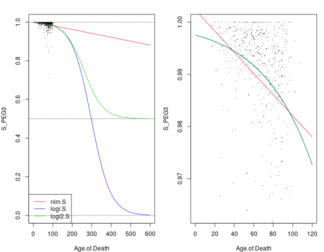
The link functions are given by the following equations
These functions are illustrated by the following plot; nlm: solid green, logi: solid red, and logi2: dashed blue. They reflect simple (univariate) regression models with as response and Age.of.Death as the only explanatory variable. Thus there are two regression coefficients in all three cases, and these were estimated with iterative weighted least squares using R’s glm function. logi and logi2 are almost indistinguishable in the range of all observed ages but become quite different around 300 years (much longer than the human lifespan).
Below printed are two measures of fit: residual deviance (top block) and AIC (bottom block). Note the negative estimated AIC for nlm.S, which is unexpected since the theoretical value of AIC for any model must be nonnegative. Subsequent analysis will investigate this discrepancy surrounding the estimated AIC.
##        nlm.R       nlm2.R        nlm.S       logi.S      logi2.S
## 4.348327e+05 4.348327e+05 2.028023e-01 5.484768e+03 1.127678e+04
## $nlm.R
## [1] 4740.081
##
## $nlm2.R
## NULL
##
## $nlm.S
## [1] -2432.414
##
## $logi.S
## [1] 7116.834
##
## $logi2.S
## [1] 13207.78
Although the models might appear freely combinable with both data transformations, it is not clear how logistic model(s) might be fitted after rank transformation of . Because how should total read counts (the weights) be transformed? But the converse case is straight-forward: to fit nlm to untransformed despite its apparent heteroscedasticity and nonlinearity (see Ifat’s plots and the data exploration below).
Therefore the three model families give rise to four types of models depending on whether the response is rank-transformed or not. These are summarized in the table below:
| nlm.R | nlm.S | logi.S | logi2.S | |
|---|---|---|---|---|
| link function | linear | linear | logistic | scaled logistic |
| response distrib. | normal (Gaussian) | normal (Gaussian) | binomial | binomial |
| response | ||||
| weights | 1 (uniform) | 1 (uniform) |
So, considering these 4 types combined with 16 genes separately, or with the two kinds of data aggregations (averaging and pooling) using 3 gene sets, each with or without filtering, there are fitted models in the present analysis.
Implementation
The multifaceted goals of the present analysis called for a completely new implementation of data manipulations and models because the earlier implementation (by Ifat) lacked the necessary modularity. The script files for the new and old implementation:
source('2016-04-22-glm-for-s-statistic.R')
source('../2016-03-02-ifats-regression-analysis/2016-03-02-ifats-regression-analysis.R')
The new code provides the function nlm for the nlm model, logi for logi, and logi2 for logi2. Additionally, the nlm2 function also implements nlm, but instead of calling R’s glm function (which is also called by logi and logi2), it calls lm. The definition of logi2 is nearly identical to logi; the only difference is using C2 as response variable instead of C. Wheres C contains the original observed “higher” and “lower” read counts, C2 is a transformation of those that corresponds to the (inverse) scaling function of the logistic functiion in logi2.
f <- list(
          nlm.R = function(y, d) { # normal linear model with rank R as response
              glm(formula = mk.form(paste0("R_", y)), family = gaussian, data = d)
          } ,
          nlm2.R = function(y, d) { # as above but with the R's lm function instead of glm
              lm(formula = mk.form(paste0("R_", y)), data = d)
          } ,
          nlm.S = function(y, d) { # normal linear model with S statistic as response
              glm(formula = mk.form(paste0("S_", y)), family = gaussian, data = d)
          } ,
          nlm2.S = function(y, d) { # as above but with the R's lm function instead of glm
              lm(formula = mk.form(paste0("S_", y)), data = d)
          } ,
          logi.S = function(y, d) { # logistic regression with the S statistic as response
              glm(formula = mk.form(paste0("C_", y)), family = binomial, data = d)
          } ,
          logi2.S = function(y, d) { # as above but with rescaled and offset logistic link function
              glm(formula = mk.form(paste0("C2_", y)), family = binomial, data = d)
          } )
As expected, all results with nlm2 were found to be identical to nlm (not shown).
Exploratory analysis
The following plots explore the relationship between a given response variable and 12 of the 13 explanatory variables (the 13th one, Ancestry.EV.5 showed no systematic relationship and is omitted here so that plots can be arranged in arrays). In this document only filtered data are presented because filtering had no visually appreciable effect on the plot.
Responses averaged across genes
When the response is the average (below), a qualitatively similar, inverse, relationship emerges between statistic and age as seen in Ifat’s plots, which depicted 13 genes separately. Some of the remaining 11 explanatory variables, like Institution or PMI.in.hours seem to effect , while others like Gender don’t.

When ranks are averaged as , the response appears more homoscedastic (its dispersion appears unaffected by explanatory variables) but some of the systematic effects that are seen without transformation (e.g. PMI.in.hours) are diminished.

Responses pooled across genes
The next set of plots shows data points for all genes pooled together rather than averaged together so each plot has many more points than before. Below are plots with as response for all 16 genes.

Below are plots with (observed ranks) as response. Compared to the corresponding results obtained with averaging there is clearly less systematic variation of the response with explanatory variables, which hints at their differential effects on various genes.

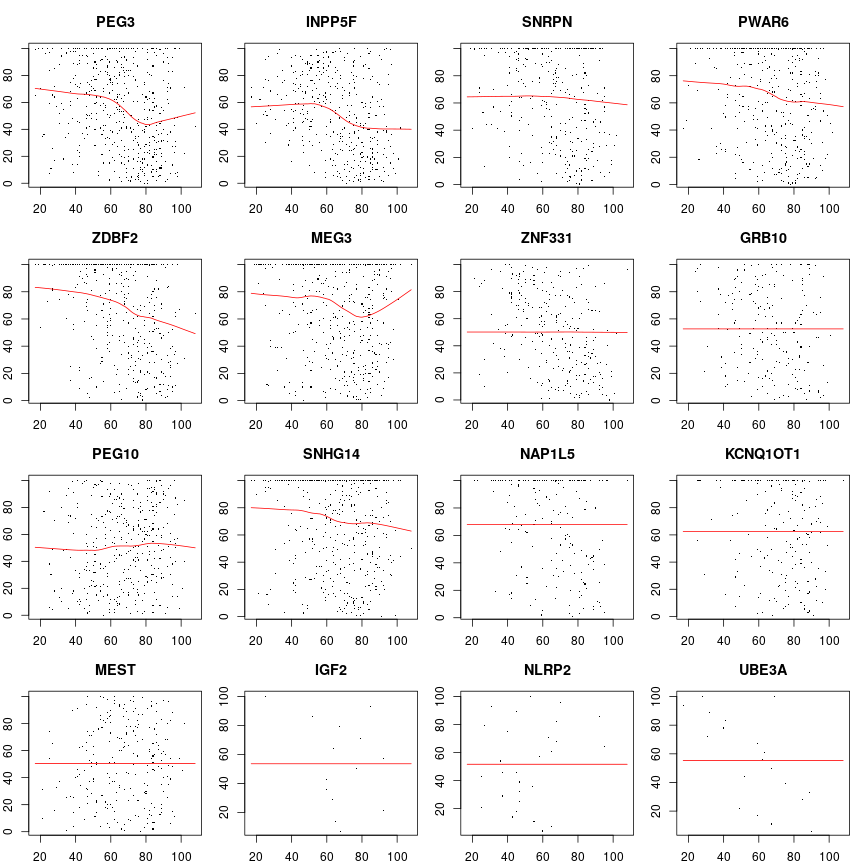
Response vs age for each gene separately
The differential effect of age on the response of various genes is illustrated now. Plotted below is the observed statistic versus age for each gene separately. Dots are data points and the solid line is the smoothed data with the Lowess filter. The lower percentile of , for each , has been trimmed off to enhance clarity. Judged from the smooth curves the effect of age appears quite small. Still, gene-to-gene variation is apparent.

Below are similar plots to the ones above but now with as response (i.e. with rank-transformation). The among genes variation is quite clear.
Conditional dependence on age given other explanatory variables
The apparent dependence of the response on age is marginal in the sense that other explanatory variables are disregarded in the previous plots. However, those other variables may induce spurious dependence between the response and age even if those are conditionally independent. Therefore, the next two sets of plots are conditioned on one of three explanatory variables, Institution, the RNA quality measure DLPFC_RNA_isolation..RIN, and Ancestry.EV.2 reporting on the population structure(?) that were found to exert highly significant effect in Ifat’s earlier regression analysis. DLPFC_RNA_isolation..RIN.2 had also highly significant effect, but it correlates so tightly with DLPFC_RNA_isolation..RIN (Pearson corr. coef 1) that it carries no additional information.
Importantly, these plots below suggest that, at least for PEG3, the response’s dependence on age seems genuine and not entirely due to confounding effects of other variables.
## Error: <text>:2:30: unexpected input
## 1: # condition R_PEG3 vs age on a given institution, RIN value and ancestry
## 2: coplot(S_PEG3 ~ Age.of.Death \
##                                 ^
Regression analysis
Comparing implementations
Let’s compare the normal linear model obtained with Ifat’s implementation to that with the new implementation! For consistency with Ifat’s previous results the data manipulations are: filtering, rank-transformation, and averaging over selected genes.
sapply( c("deviance", "aic", "coefficients"), function(s) all.equal(m.ifat.avg8[[s]], m$avg8$nlm.R[[s]]))
##                                deviance
##  "Mean relative difference: 0.04045548"
##                                     aic
## "Mean relative difference: 0.004622527"
##                            coefficients
##  "Mean relative difference: 0.02769083"
These results show a close but not perfect match between the old and new implementation. The slight discrepancy seems to be due to a rounding step in the old code, for which I found no justification and therefore omitted from the new implementation.
Effect of filtering
Filtering out “noisy” observations (those with low total read counts) is expected to improve model fit to data. When too few points are retained after filtering, overfitting may occur. This is illustrated by the plots below, where filtering induces extremely large improvement for genes with scarce data, like IGF2 or NLRP2. Improvement is expressed as minus relative AIC defined as , where indicates filtering and no filtering.
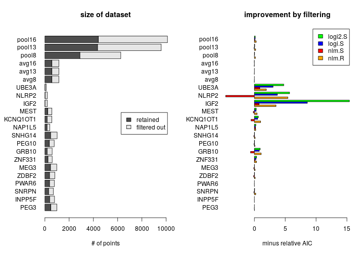
All results presented in this document were obtained with filtering unless otherwise noted.
To what extent is the apparent effect of age confounded?
The previous conditional plots of vs age qualitatively examined the extent of confounding by three additional variables such as Institution. The regression coefficient under some model reports the effect of age on the response. In simple regression is estimated from a model where the linear predictor contains only age so that . Then the additional variables behave as latent variables confounding the effect of age. Multiple regression includes these additional variables in the linear predictor removes their confounding effect from .
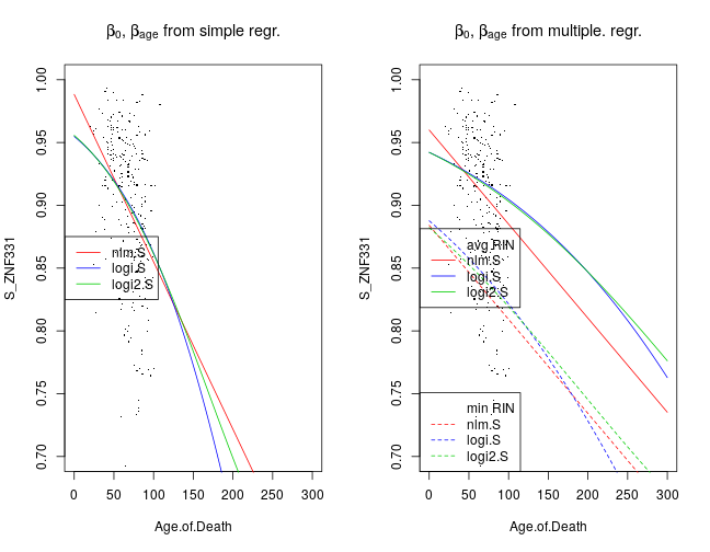
Here I compare estimated from simple and multiple regression under the nlm.S, logi.S and logi2.S model types. First let’s return to the earlier plot of fitted simple regression models to the and data. Given a model family such as nlm, the mean of is a function of and as well as estimated from simple regression, shown by the left graph. This function is changed when are estimated from multiple regression together with 21 other regression coefficients (right panel). For instance, and mediate the effects of RNA quality measures and . Two fitted curves are shown for each model: the solid lines correspond to the case when and that is the average of the observed and across all individuals , respectively; on the other hand, the dashed lines correspond to and .
The main point, though, is that for any given model the estimated from multiple regression is less negative in that from simple regression. This appears visually as shallower fitted curves. The interpretation is that a large confounding effect by other variables was removed by multiple regression.
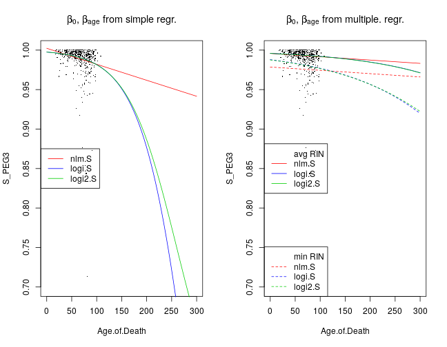
The changes in the fitted curves are qualitatively similar for all genes and aggregated gene sets. ZNF331 shows the most profound effect of age on after the removal of the confounding effects by multiple regression.
The effect of age with and without correction for confounding
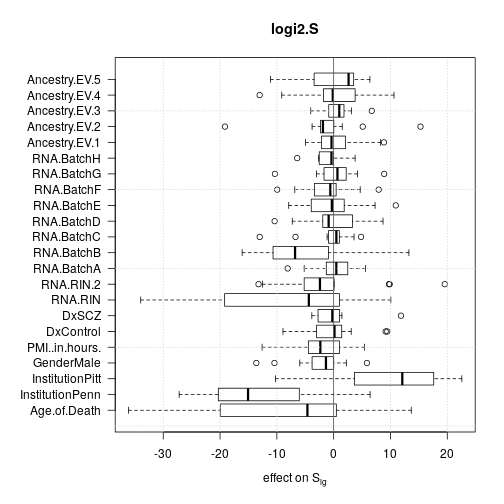
The following set of plots compares estimates of from the simple (dark grey) and multiple (light grey) regression under various model families. These results can be summarized as
- age has a negative effect on the response (loss of imprinting)
- based on multiple regression, the estimated effect size and significance of age is smaller, which indicates substantial confounding in simple regression
- for genes with scarce data the effect size can be large without being significantly different from zero
nlm.R
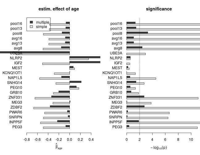
nlm.S
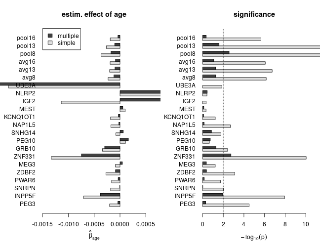
logi.S
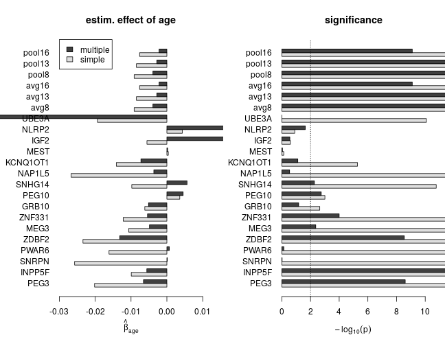
logi2.S
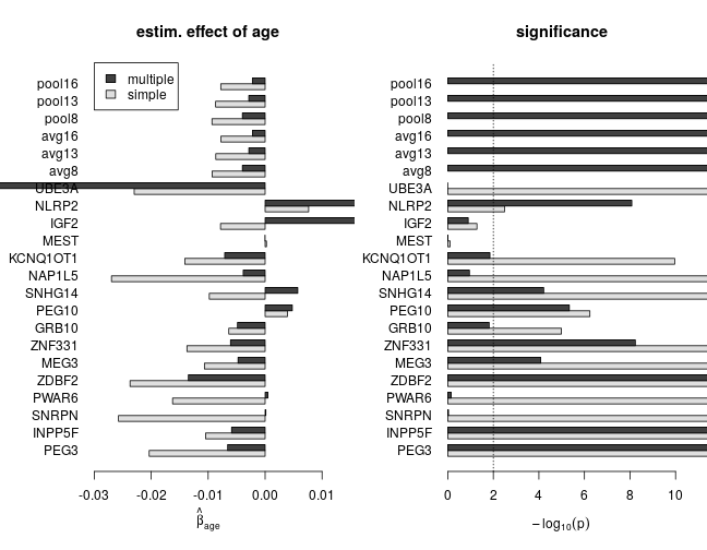
Gain of imprinting?
The above results suggest gain of imprinting with age for PEG10 and SNHG14 under all multiple regression models, although with varying effect size and significance. Below are the p-values for
signif(sapply(m$PEG10, function(x) summary(x)$coefficients['Age.of.Death', 4]), digit=2)
##   nlm.R  nlm2.R   nlm.S  nlm2.S  logi.S logi2.S
## 2.8e-01 2.8e-01 1.8e-01 1.8e-01 1.8e-03 4.6e-06
signif(sapply(m$SNHG14, function(x) summary(x)$coefficients['Age.of.Death', 4]), digit=2)
##   nlm.R  nlm2.R   nlm.S  nlm2.S  logi.S logi2.S
## 3.6e-02 3.6e-02 1.4e-01 1.4e-01 5.3e-03 6.1e-05
Relative effects of explanatory variables
This section presents the relative impact of explanatory variables using two ways. Effects decomposes the observed response vector (, or ) to orthogonal components, where the first components are associated with the coefficients . Deviance from ANOVA is the second way: this partitions systematic variation according to explanatory variables. Note that there are fewer explanatory variables than coefficients (due to some explanatory variables being factors) and that effects provides directional information but deviance does not. Despite this difference, the results show good overall agreement between effects and deviance.
Both for effects and deviance 13 genes were used discarding the 3 genes with scarce data.
Effects
The following set of plots present effects of regression models using the effects function of R. Explanation from the documentation of effects:
For a linear model fitted by lm or aov, the effects are the uncorrelated single-degree-of-freedom values obtained by projecting the data onto the successive orthogonal subspaces generated by the QR decomposition during the fitting process. The first r (the rank of the model) are associated with coefficients and the remainder span the space of residuals (but are not associated with particular residuals).
For each effect all 13 single genes data sets were used but aggregated data sets were discarded to avoid redundancy. The plots show that age and institution have the largest effects but RNA quality and RNA library batch are prominent as well.
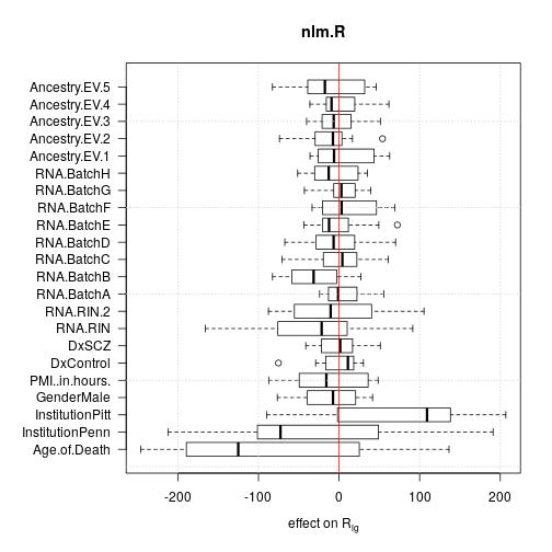
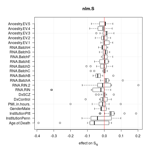
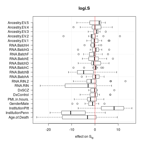
Deviance from ANOVA


Conclusions
- age has a moderate but significant negative effect on parental bias “response” measured by
- some of the other explanatory variables (Institution, RIN) have highly significant effect with size comparable to that of age; therefore these variables confound simple regression on age or visual inspection of age vs. plots
- this confounding is corrected for by multiple regression
- these findings hold under all model types (nlm, logi and logi2)
- the next question is how models compare to each other and which one should be selected