Lab Notebook

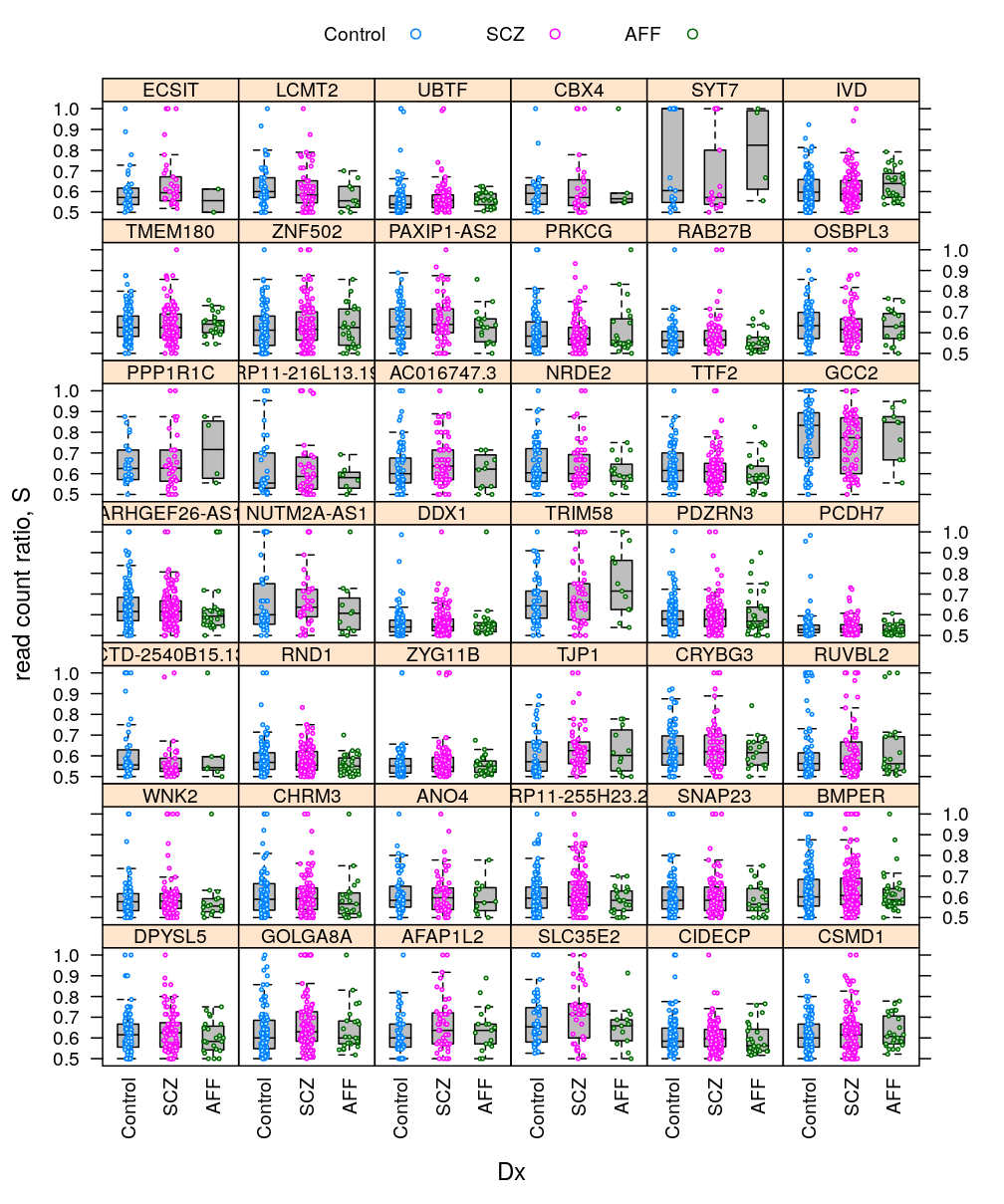
Various plots present the distribution of read count ratio across individuals and genes jointly. Genes are also ranked using a summary statistic derived from the empirical distribution of read count ration across individuals for each given gene.

Missing data due to bug

For each gene $g$ of 16026 genes the higher and lower read counts across $I_g\le 579$ individuals $\{H_{ig}, L_{ig} \,\mid \, i=1,...,I_g\}$ are stored in a .csv file. However, nearly 3 % of those files are empty due to a bug that resulted in multiple headers in Ifat’s html tables (see for instance gene AK3) and to the inability of my converter script to deal with such tables. To see this:

DATADIR="../../data/readcount/"
SEDCMD='s/^.*attila attila\s\+\([[:digit:]]\+\).*\/\([^/]\+\)\.csv$/\1,\2/'
OUTFILE="${DATADIR}/fsize-genes.csv"
[ -f $OUTFILE ] || {
    # create header
    echo "file.size,gene.symbol" > $OUTFILE
    # get file size (in bytes) for each gene under 'genes' directory
    find "${DATADIR}/genes" -name '*.csv' | xargs ls -l | sed "$SEDCMD" >> $OUTFILE
}
cat <<EOF
Number of .csv files

all: $(grep --count '^[[:digit:]]\+,' $OUTFILE )
empty: $(grep --count '^0,' $OUTFILE )
EOF

## Number of .csv files
## 
## all: 16026
## empty: 442

## Loading required package: RColorBrewer

Import read count data

Load data importer functions:

source("../../src/import-data.R")
source("../../src/utils.R")
source("2016-07-19-genome-wide-S.R")

The following expressions import $S_{ig}$ for all 1.5584 × 10⁴ genes for which the csv file is nonempty.

gene.summary <-
    read.csv("../../data/readcount/summary-all-genes.csv")
rownames(gene.summary) <- gene.summary$Symbol
gene.summary$file.size <-
    read.csv("../../data/readcount/fsize-genes.csv", row.names = 2)[rownames(gene.summary), , drop = TRUE]
gene.ids <- with(gene.summary, as.character(Symbol)[ file.size > 0 ])

Y <- get.readcounts(gene.ids, g.subsets = list(), sel.var = c("H", "N"), rm.conflict = TRUE)
S <- data.frame(lapply(gene.ids, function(g) Y[[g]]$H / Y[[g]]$N), check.names = FALSE)
names(S) <- gene.ids
N <- data.frame(lapply(Y, getElement, "N"), check.names = FALSE)
rm(Y)

Perform filtering

Filtering genes based on number of observations

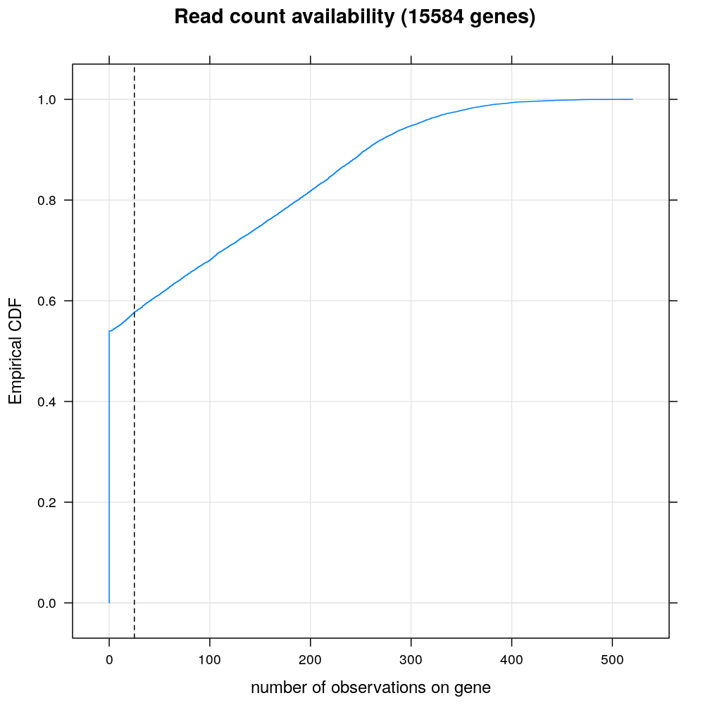
For more than half of even the genes $g$ with nonempty files the number $I_g$ of observations (the number of individuals/RNA samples with read count data on $g$) is zero. In what follows, not only these genes are filtered out but also those with less than 10 observations, indicated by the vertical dashed line on the empirical ECDF plot below.

min.n.obs <- 25

Data preparation

Update: filtering based on a subsequent post

min.obs <- 25 # reset t_ind
# implementation detail!: filter out genes with fewer observations than 'min.obs'
g.passed <- names(S)[sapply(S, function(y) sum(! is.na(y)) >= min.obs)]
min.reads <- 15 # set t_rc
S <- filter.min.read(min.reads, X = S[g.passed], N = N[g.passed], min.obs = min.obs)
N <- filter.min.read(min.reads, X = N[g.passed], N = N[g.passed], min.obs = min.obs)
# ECDFs for all filter levels and all genes g; individual ECDF components F_g are named according to gene g
# the expression also sorts genes g according to F_g(0.9) where F_g is the ECDF for gene g 
ED <- list(fun = sorted.ecdfs(S))
# evaluate ECDF at
ED$ss <- seq(0.5, 1, length.out = 101)
ED$val <- data.frame(lapply(ED$fun, function(f) f(ED$ss)), check.names = FALSE)
# fractions of interest
frac <- do.fractions(ED$fun, S, N, frac = 10:6 / 10,
                     ucl.fun = CI.p, max.ucl = 0.7, max.s = 0.6)
# sort data according to gene ranking
S <- S[names(ED$fun)]
N <- N[names(ED$fun)]

Computationally demanding calculations to prepare data for presentation:

ED.long <- reshape(ED$val, v.names = "ECDF", varying = names(ED$val),
                   timevar = "gene", times = factor(names(ED$val)),
                   idvar = "s", ids = ED$ss, direction = "long")
ED.long$gene <- factor(ED.long$gene, levels = names(ED$val), ordered = TRUE)

Figure for manuscript

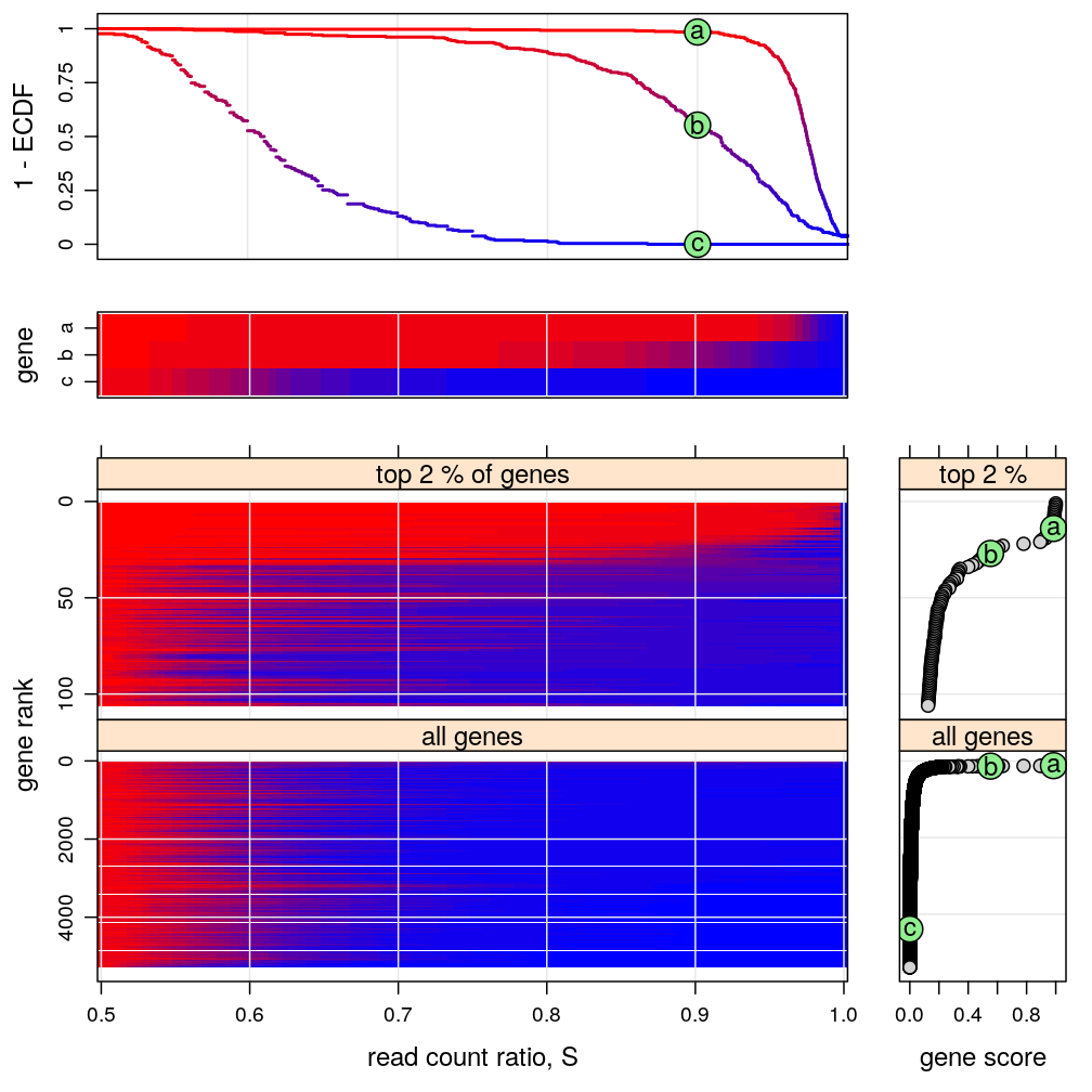
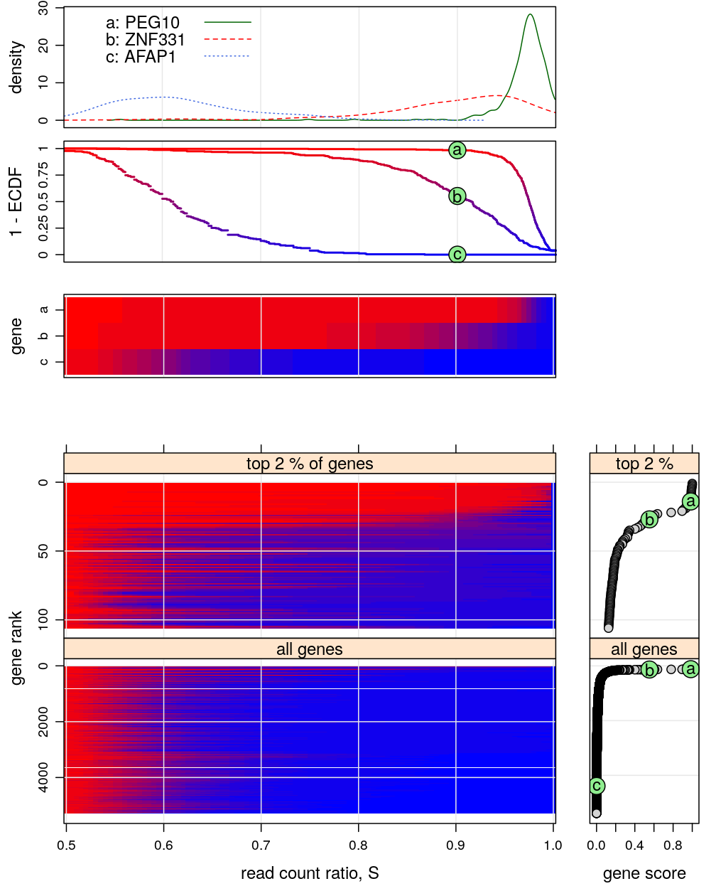
This figure is intended to:

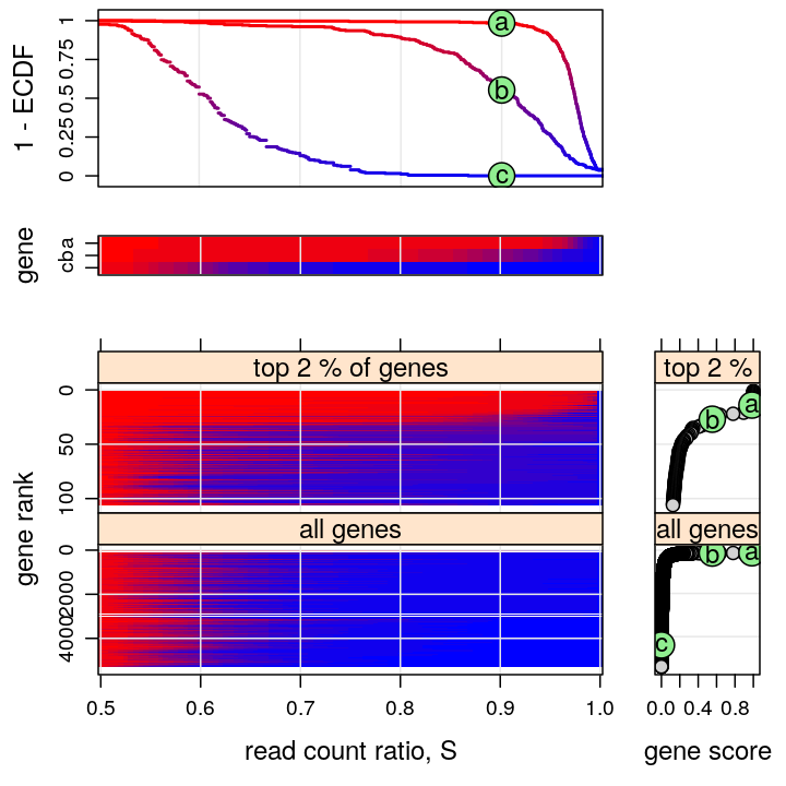
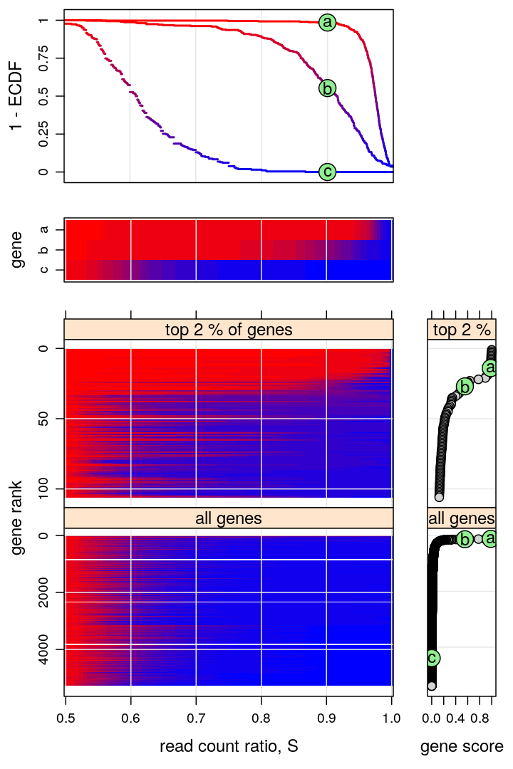
• present a few representative genes characterized by the “read count ratio” statistic $S$ (two upper graphs)
  • e.g. PEG10 and ZNF331 represent monoallelic expression and AFAP1 biallelic expression
    1. density est.: kernel density estimates, whose interpretation is identical to that of histograms
    2. ECDF: empirical cumulative distribution function, sometimes called cumulative fraction
• present a compact genome-wide overview of parental imbalance (lower left graph)
  • imbalance is expressed in terms of the ECDF of $S$ using a color scheme, introduced in the upper 2nd and 3rd graphs
  • the thousands of genes are ranked from the most imbalanced (monoallelic, top) to the most balanced (biallelic, bottom)
  • the ranking is based on the ECDF evaluated at $s = 0.9$, as shown in the upper 2nd graph and the bottom right plots
• support the conclusion that $\approx 1 \%$ of all genes are appreciably imbalanced (monoallelically expressed)

There are 5283 genes on this figure but before filtering there were 15584 genes.

Figures for live presentation

Revision for Nature Communications

source("../../src/fit-glms.R")
set.seed(19760415) # my birthdate
sel.g.rnd <- sample(names(S), 42)
Y.long <- reshape.Y2long(sel.g.rnd)