Lab Notebook

It is crucial for publication to ensure that the genes selected for regression analysis were chosen on objective criteria. This requires the reproduction of the set of genes that were called monoallelic in the manuscript drafted by Ifat. I’ll refer to that in this document as the previous manuscript. If perfect reproduction fails then minimum discordance is desired, and the regression analysis will potentially need to be repeated accordingly with the new set of genes called monoallelic.

This post was extended with the test for reference/nonreference bias, whose results are summarized in ref-nonref-test.csv for top scoring genes.

Procedures from the previous manuscript

Filters

The previous manuscript makes several statements on how the data were filtered before the gene were ranked and presented on Fig 1:

section Methods: Allelic expression analyses, p3

there had to be $\ge 7$ reads, with a quality score $\ge 20$; a further gene-wide filter requires $20$ or more such reads for the gene to be assessable in a given individual

section Methods: Allelic expression analyses, p4

Genes that were supported by fewer than 25 subjects were excluded.

section Results: Pipeline, p4

there had to be $\ge 7$ reads; a further gene-wide filter requires 15 or more such reads for the gene to be assessable in a given individual

section Results: Landscape of monoallelic expression[…], p6

sufficient coverage defined as $\gt 20$ reads mapping to heterozygous SNPs per individual in at least ten individuals

In addition, for the regression analysis a stronger filtering was used:

section Results: Relaxation of imprinting, p8

We examined genes where we had greater than 180 analyzable individuals and where 30% or more of those individuals displayed monoallelic expression defined by Sg >0.9. An analyzable individual was defined as one with at least 50 reads at one or more SNPs imputed to be heterozygous (Lhet cutoff of 0.95 as above).

My interpretation

Two kind of filters were used: I call them read count-based and individual-based. These have the following properties:

1. the read count-based filter removes any such pair $(i,g)$ of individual $i$ and genes $g$ for which the total read count $n_{ig}<t_\mathrm{rc}$, where $t_\mathrm{rc}$ is what I call a read count threshold
   • Note that there is another read count-based filter, which removes pairs $(s,g)$ of SNP $s$ and gene $g$ in the same fashion as the previous one but with threshold 7. However, I cannot investigate this filter until the SNP-wise read counts become easily accessible.
2. the individual-based filter removes any genes $g$ (across all individuals) if read count data involving $g$ are available on less than $t_\mathrm{ind}$ number of individuals

Note that in fact there are two read count-based filters: not only the one for individual SNPs and a

Given the above quotations from the previous manuscript the read count-based filter might have been applied with $t_\mathrm{rc} = 20 \text{ or } 15 \text{ or } 21$, whereas the individual-based filter with $t_\mathrm{ind} = 25 \text{ or } 10$ in order to arrive at Fig 1.

Ranking and calling monoallelic expression

The ranking of genes is based on the following score. The score of gene $g$ is the fractions of individuals $i$ for whom $s_{ig} \gt 0.9$. In other words the score of $g$ is based on the empirical cumulative distribution function ECDF $\hat{F}_g$ or, equivalently, on the survival function $1-\hat{F}_g$: $\text{the score of gene } g = 1 - \hat{F}_g(0.9).$

Judged from Fig 1 the classification of genes appears to have been defined as follows: $\text{the score of gene } g \ge 0.3 \Rightarrow g$ is called monoallelic. Otherwise $g$ is called not monoallelic. (Does “not monoallelic” imply biallelicity or do we wish to consider one or more intermediate classes?) However, nothing is explicitly stated in the previous manuscript on the classification of genes independently of individuals. For example (section Results: Landscape of monoallelic expression[…], p6) we read

1b shows the 13 (of 32) genes that did not make it into the top Sg scoring group

but we are not told the criterion based on which the top scoring group was defined.

Other quantities of interest

Although not used for ranking or classification, other fractions were also calculated and presented in Fig 1. First, not only $\hat{F}_g(s=0.9)$ was obtained but also $\hat{F}_g(s)$ for $s = 0.6,0.7,0.8$. Second, the fraction of individuals were calculated that passes the test conceived by Andy: $\text{given gene } g \text{ the fraction of indiv. passed} = \frac{\# \{i \,:\, s_{ig} \le 0.6 \text{ and } \mathrm{UCL}_{ig} \le 0.7 \}}{\# \{i\}},$ where the upper 95 % confidence limit is given by $\mathrm{UCL}_{ig} = s_{ig} + z_{0.975} \sqrt{\frac{s_{ig} (1 - s_{ig})}{n_{ig}}},$ such that $z_{p}$ is the $p$ quantile of the standard normal distribution and $n_{ig}$ is the observed total read count.

Results

Genome-wide data import and preparation

## Loading required package: RColorBrewer

Load functions:

source("../../src/import-data.R")
source("../../src/utils.R")

Read count data have been imported (not shown). We see that the minimum number of reads for any gene and individual is 7.

min(unlist(N), na.rm = TRUE)

## [1] 7

The following code

1. applies “a filter giving priority to even a single SNP showing biallelic expression” (see Ifat’s ms and her “1_conflict” annotation)
2. applies the read count-based filter given a sequence of read count thresholds $t_\mathrm{rc}$
3. applies the individual-based filter given $t_\mathrm{ind}$
4. calculates the fractions of interest, which include the score $1-\hat{F}_g(0.9)$
5. ranks genes according to their score

min.obs <- 25 # set t_ind
# implementation detail!: filter out genes with fewer observations than 'min.obs'
g.passed <- names(S)[sapply(S, function(y) sum(! is.na(y)) >= min.obs)]
# a sequence of thresholds t_rc for minimum read count to filter individual data points S_{ig} or N_{ig}
min.reads <- c(7, 15, 20)
min.r.names <- paste0("min.reads.", min.reads)
names(min.r.names) <- min.r.names
names(min.reads) <- min.r.names
# filter S_{ig} (then N_{ig}) first based on 'min.reads' and then again on 'min.obs'
Sf <- lapply(min.reads, function(m) filter.min.read(m, X = S[g.passed], N = N[g.passed], min.obs = min.obs))
Nf <- lapply(min.reads, function(m) filter.min.read(m, X = N[g.passed], N = N[g.passed], min.obs = min.obs))
# ECDFs for all filter levels and all genes g; individual ECDF components F_g are named according to gene g
ECDF <- lapply(Sf, sorted.ecdfs)
frac <- lapply(min.r.names,
               function(m)
                   do.fractions(ECDF[[m]], Sf[[m]], Nf[[m]],
                                frac = 10:6 / 10, ucl.fun = CI.p, max.ucl = 0.7, max.s = 0.6))

Note that the individual-based filter is also applied before the read count-based one. However, this step is an implementation detail and has no conceptual significance.

Result on the individual-based filter

Besides $t_\mathrm{ind}=25$ the threshold $t_\mathrm{ind}=10$ was also tested (not shown) but the former resulted in clearly more consistency with Ifat’s ranking (see below).

Gene rankings

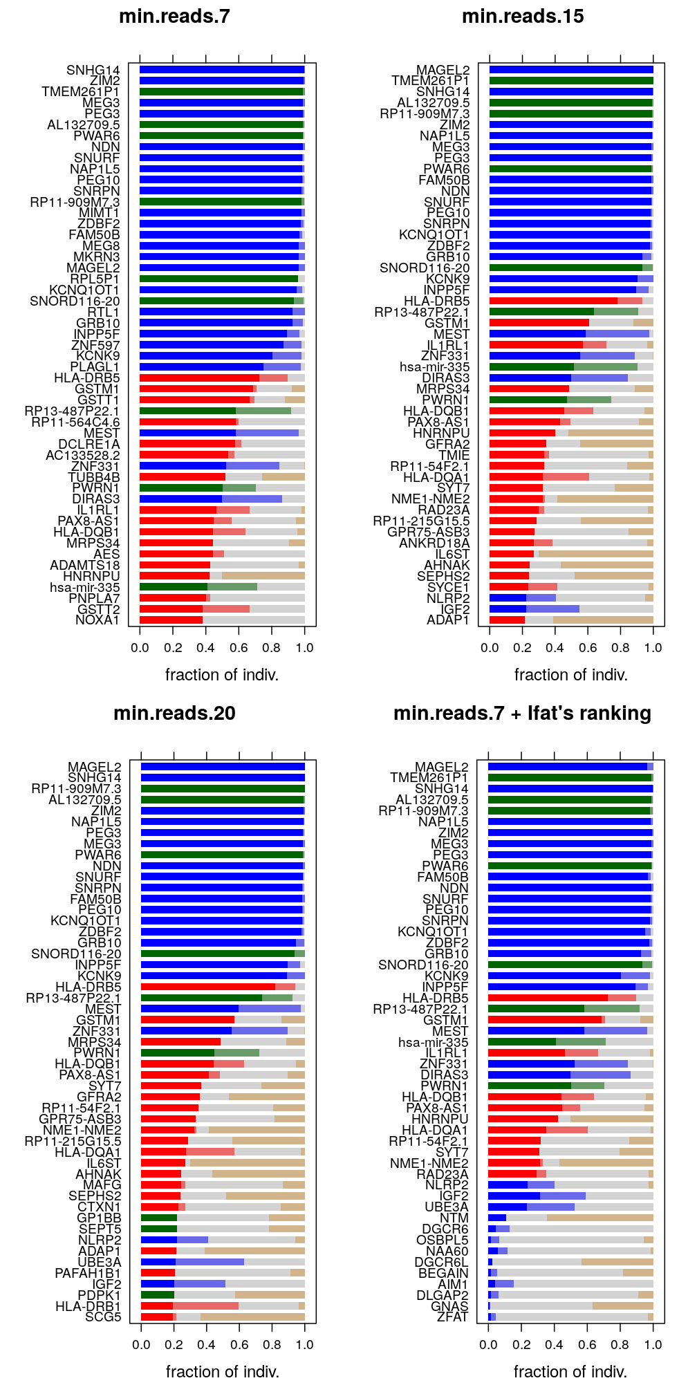
The plots show four gene rankings and the corresponding fractions of interest. The first three correspond to the sequence of three $t_\mathrm{rc}$ settings of the read count-based filter so these rankings will be named $R_{7}, R_{15}, R_{20}$. The fourth plot follows the ranking seen on Ifat’s Fig 1, and this ranking will be referred to as $R_\mathrm{Ifat}$. Since that figure shows only the 51 genes, the same is done here for also the first three plots. Note that the last 13 genes of the fourth plot are in fact low ranking “known” imprinted genes so they are not in the top 51 according to $R_\mathrm{ifat}$. The first three plots do, however, present the 51 top ranking genes for the corresponding ranking.

Figure for manuscript

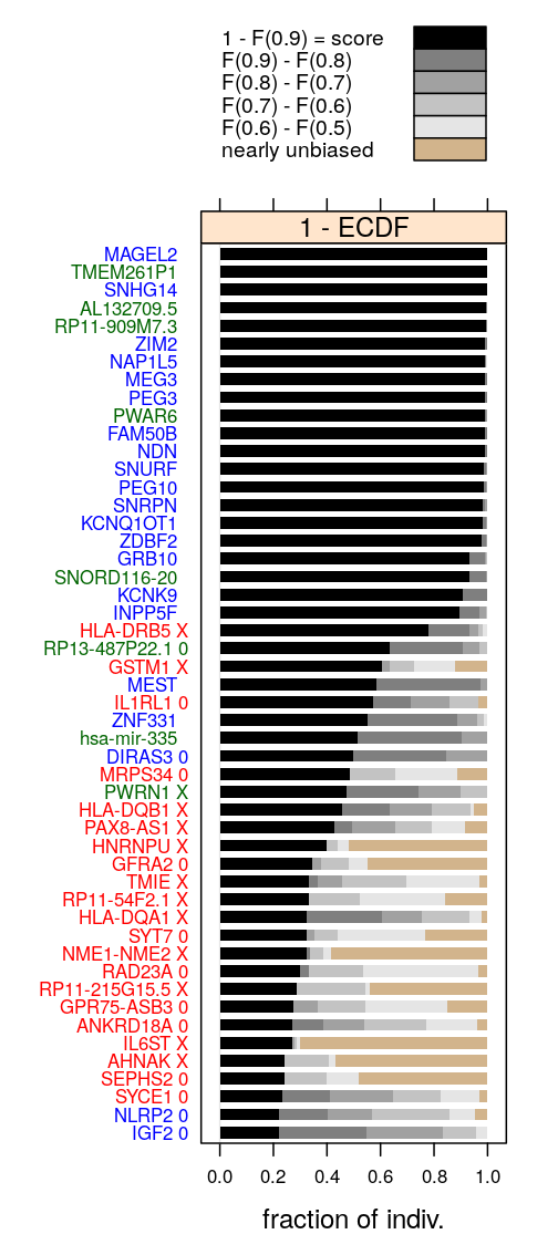
The basis for the figure is the one in the upper-right panel in the previous plot, which is supplemented with the outcome of the “reference/non-reference allele bias” test. The outcome was done via a subjective analysis by Andy and I, in which we sorted each of the top 51 genes into three categories: biased, unbiased, and indeterminate. These are stored in ref-nonref-test.csv and correspond to X, ` ` (whitespace) and 0 in ref.allele.bias, respectively:

ref.allele.bias <- read.csv("../../results/ref-nonref-test.csv")$ref.allele.bias[1:50]
names(ref.allele.bias) <- read.csv("../../results/ref-nonref-test.csv")$gene[1:50]
levels(ref.allele.bias) <- c("X", "0", " ")

Gene rankings with Ifat’s ranking as reference

The previous figures show that several genes in the top 51 according to $R_{7}, R_{15}$ or $R_{20}$ are missing from Ifat’s figure. But clearly, when the read count-based filter is used at $t_\mathrm{rc}=15$ there is a close match with Ifat’s ranking.

##               imprinting.status R.ifat  R.7 R.15 R.20
## MAGEL2          known imprinted      1   19    1    1
## TMEM261P1      nearby candidate      2    3    2   NA
## SNHG14          known imprinted      3    1    3    2
## AL132709.5     nearby candidate      4    6    4    4
## RP11-909M7.3   nearby candidate      5   13    5    3
## NAP1L5          known imprinted      6   10    7    6
## ZIM2            known imprinted      7    2    6    5
## MEG3            known imprinted      8    4    8    8
## PEG3            known imprinted      9    5    9    7
## PWAR6          nearby candidate     10    7   10    9
## FAM50B          known imprinted     11   16   11   13
## NDN             known imprinted     12    8   12   10
## SNURF           known imprinted     13    9   13   11
## PEG10           known imprinted     14   11   14   14
## SNRPN           known imprinted     15   12   15   12
## KCNQ1OT1        known imprinted     16   21   16   15
## ZDBF2           known imprinted     17   15   17   16
## GRB10           known imprinted     18   24   18   17
## SNORD116-20    nearby candidate     19   22   19   18
## KCNK9           known imprinted     20   27   20   20
## INPP5F          known imprinted     21   25   21   19
## HLA-DRB5      distant candidate     22   29   22   21
## RP13-487P22.1  nearby candidate     23   32   23   22
## GSTM1         distant candidate     24   30   24   24
## MEST            known imprinted     25   34   25   23
## hsa-mir-335    nearby candidate     26   48   28   NA
## IL1RL1        distant candidate     27   41   26   NA
## ZNF331          known imprinted     28   37   27   25
## DIRAS3          known imprinted     29   40   29   NA
## PWRN1          nearby candidate     30   39   31   27
## HLA-DQB1      distant candidate     31   43   32   28
## PAX8-AS1      distant candidate     32   42   33   29
## HNRNPU        distant candidate     33   47   34   NA
## HLA-DQA1      distant candidate     34   57   38   36
## RP11-54F2.1   distant candidate     35   61   37   32
## SYT7          distant candidate     36   65   39   30
## NME1-NME2     distant candidate     37   63   40   34
## RAD23A        distant candidate     38   69   41   NA
## NLRP2           known imprinted     NA   89   49   44
## IGF2            known imprinted     NA   64   50   48
## UBE3A           known imprinted     NA   92   60   46
## NTM             known imprinted     NA  335  138  106
## DGCR6           known imprinted     NA 1306  646   NA
## OSBPL5          known imprinted     NA 3652  987 1009
## NAA60           known imprinted     NA  904 1238 1341
## DGCR6L          known imprinted     NA 2809 1332 1030
## BEGAIN          known imprinted     NA 4215 1378 1383
## AIM1            known imprinted     NA 1534 3600   NA
## DLGAP2          known imprinted     NA 3691 3526 3171
## GNAS            known imprinted     NA 5816 4699 4148
## ZFAT            known imprinted     NA 3924 4595 4044

In fact, the two rankings agree for the top 24 genes (except that ranks 6 and 7 are swapped):

all.equal(genes.ifat.ranks[ , "R.15"][c(1:5, 7:6, 8:24)], 1:24)

## [1] TRUE

From this result we may conclude that Ifat’s filter settings were $t_\mathrm{rc}=15$ and $t_\mathrm{ind}=25$ and the discrepancies we see might partly or entirely be due to rounding errors introduced at the export of $S$ values to csv files and/or different implementation of the calculation of gene scores.

Monoallelically called genes

Given the result that $R_{15}$ resembles the most to $R_\mathrm{ifat}$, we will use $R_{15}$ to call monoallelic genes. We will compare called gene sets under different threshold for the score $1 - \hat{F}_g(0.9)$ and further compare these to the one presented in the previous manuscript.

Notice that the lowest scoring gene in the “nearby candidate” category is PWRN1 (green on Fig 1). Its score is 0.4714286 and it ranks at 31 according to $R_{15}$ and at genes.ifat.ranks["PWRN1", "R.ifat"]. We may define the classification threshold such that we only call genes monoallelic if their score $\ge0.4$:

(called.mono.0.4 <- names(frac$min.reads.15)[unlist(frac$min.reads.15[1, ]) >= 0.4])

##  [1] "MAGEL2"        "TMEM261P1"     "SNHG14"        "AL132709.5"   
##  [5] "RP11-909M7.3"  "ZIM2"          "NAP1L5"        "MEG3"         
##  [9] "PEG3"          "PWAR6"         "FAM50B"        "NDN"          
## [13] "SNURF"         "PEG10"         "SNRPN"         "KCNQ1OT1"     
## [17] "ZDBF2"         "GRB10"         "SNORD116-20"   "KCNK9"        
## [21] "INPP5F"        "HLA-DRB5"      "RP13-487P22.1" "GSTM1"        
## [25] "MEST"          "IL1RL1"        "ZNF331"        "hsa-mir-335"  
## [29] "DIRAS3"        "MRPS34"        "PWRN1"         "HLA-DQB1"     
## [33] "PAX8-AS1"      "HNRNPU"

If we further lower the classification threshold to $0.3$ then according to $R_{15}$ several more genes must also be called monoallelic.

called.mono.0.3 <- names(frac$min.reads.15)[unlist(frac$min.reads.15[1, ]) >= 0.3]
length(setdiff(called.mono.0.3, called.mono.0.4))

## [1] 7

The upper right panel of the figure above indicates that most—if not all—of the genes between score 0.3 and 0.5 fall in the “distant candidate” category. More on this in the next section.

Implications for regression analysis

My latest regression analysis was carried out on the following genes extending the set of 8 genes initially used in the previous manuscript:

genes.regression.ifat <-
    c("PEG3", "INPP5F", "SNRPN", "PWAR6", "ZDBF2", "MEG3", "ZNF331", "GRB10", # 8 genes analyzed by Ifat
      "PEG10", "SNHG14", "NAP1L5", "KCNQ1OT1", "MEST", # 5 more genes analyzed by AGK 3/2/16
      "IGF2", "NLRP2", "UBE3A", # 3 more genes present in data files
      "TMEM261P1", "AL132709.5", "RP11-909M7.3", "SNORD116-20", "RP13-487P22.1", "hsa-mir-335", "PWRN1") # 'green' novel 1 MB imprinted genes; note that PWAR6 is already included above

These were selected based on two rules:

1. most monoallelically called genes with imprinting status either “known imprinted” or “nearby candidate”
   • exceptions include MAGEL2 and ZIM2—it is not clear why those were not selected initally or later so now they will become selected ones
2. the highest scoring but not monoallelically called “known” imprinted genes; these were IGF2, NLRP2 and UBE3A

Given these rules and the called gene sets (at score threshold 0.5 or 0.3) what genes, if any, should I extend my latest (already extended) regression analysis?

I start with the first rule. Excluding “distant candidate”s from the set of monoallelically called genes confirms the earlier suspicion that all genes scoring between 0.3 and 0.4 must be then excluded so for regression analysis it is immaterial which score is used as classfication threshold.

genes.not.cand.4 <- called.mono.0.4[gene.summary[called.mono.0.4, "imprinting.status"] != "distant candidate"]
genes.not.cand.3 <- called.mono.0.3[gene.summary[called.mono.0.3, "imprinting.status"] != "distant candidate"]
all.equal(genes.not.cand.3, genes.not.cand.4)

## [1] TRUE

To see which genes might be selected according to the second rule:

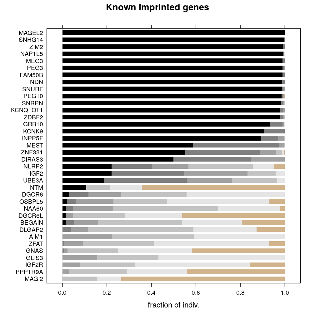
frac$min.reads.15.known <- frac$min.reads.15[gene.summary[names(frac$min.reads.15), "imprinting.status"] == "known imprinted"]
barchart(padded.frac(fr = frac$min.reads.15.known[length(frac$min.reads.15.known):1]),
              par.settings = par.set, main = "Known imprinted genes", xlab = xlab)

So, it still seems reasonable to select IGF2, NLRP2 and UBE3A based on the second rule.

Then the set of genes to carry out regression analysis:

(genes.regression.new <- c(genes.not.cand.4, c("IGF2", "NLRP2", "UBE3A")))

##  [1] "MAGEL2"        "TMEM261P1"     "SNHG14"        "AL132709.5"   
##  [5] "RP11-909M7.3"  "ZIM2"          "NAP1L5"        "MEG3"         
##  [9] "PEG3"          "PWAR6"         "FAM50B"        "NDN"          
## [13] "SNURF"         "PEG10"         "SNRPN"         "KCNQ1OT1"     
## [17] "ZDBF2"         "GRB10"         "SNORD116-20"   "KCNK9"        
## [21] "INPP5F"        "RP13-487P22.1" "MEST"          "ZNF331"       
## [25] "hsa-mir-335"   "DIRAS3"        "PWRN1"         "IGF2"         
## [29] "NLRP2"         "UBE3A"

write.csv(data.frame(genes.regression.new), file = "../../data/genes.regression.new", row.names = FALSE)

No genes need to be removed from the previous set but several new genes need to be added:

setdiff(genes.regression.ifat, genes.regression.new) # what genes to remove?

## character(0)

setdiff(genes.regression.new, genes.regression.ifat) # what genes to add?

## [1] "MAGEL2" "ZIM2"   "FAM50B" "NDN"    "SNURF"  "KCNK9"  "DIRAS3"

Cumulative loss of data

The VennDiagram package implements scaled Euler diagrams.

library(VennDiagram)

## Error in library(VennDiagram): there is no package called 'VennDiagram'

The partitions induced by filtering and calling genes monoallelic (imprinted) are illustrated by the following Euler or Venn diagrams. Note that, for an Euler diagram but not for a Venn diagram, the shapes (circles or ellipses) are proportional to the size of the set they represent and that topological relationship among shapes is such that there is no overlap if the intersection of the corresponding sets is the empty set $\{\}$.

g.sets <- list(in.dataset = 1:22254, passed.initial.filter = names(S), passed.final.filter = names(Sf$min.reads.15), called.imprinted = genes.regression.new)
sapply(g.sets, length)

##            in.dataset passed.initial.filter   passed.final.filter 
##                 22254                 15584                  5283 
##      called.imprinted 
##                    30

l <- c(n.sets <- lapply(g.sets[-4], length), n.sets[-1], rep(n.sets[3], 2))
names(l) <- NULL
l <- c(l, list(category = gsub("\\.", " ", names(g.sets[-4])), cat.cex = 1.2, cat.pos = 0, cat.dist = 1e-2))
grid.draw(do.call(draw.triple.venn, l))

## Error in grid.draw(do.call(draw.triple.venn, l)): could not find function "grid.draw"

## Error in grid.draw(do.call(draw.triple.venn, l)): could not find function "grid.draw"

## Error in grid.draw(do.call(draw.quad.venn, l)): could not find function "grid.draw"

Conclusion

• Ifat’s ranking is the most consistent with the present $R_{15}$ ranking obtained with filter settings were $t_\mathrm{rc}=15$ and $t_\mathrm{ind}=25$
• the consistency is not perfect, which might be due to implementation details
• therefore the two ranking leads to discrepant sets of monoallelically called genes
• the level of discrepancy depends on what rule is chosen for classification
• several considerations play role in what genes are seleceted for regression analysis; these have been discussed above
• the regression analysis needs to be further extended with MAGEL2, ZIM2, FAM50B, NDN, SNURF, KCNK9 and DIRAS3