Imprinted genes form clusters of one or more genes. Previous work by Ifat established the imprinting status of each gene as either known to be imprinted, not known to be imprinted but near an “known” gene, or else neither. I refer to these three categories as “known”, “nearby candidate” and “candidate”, respectively.
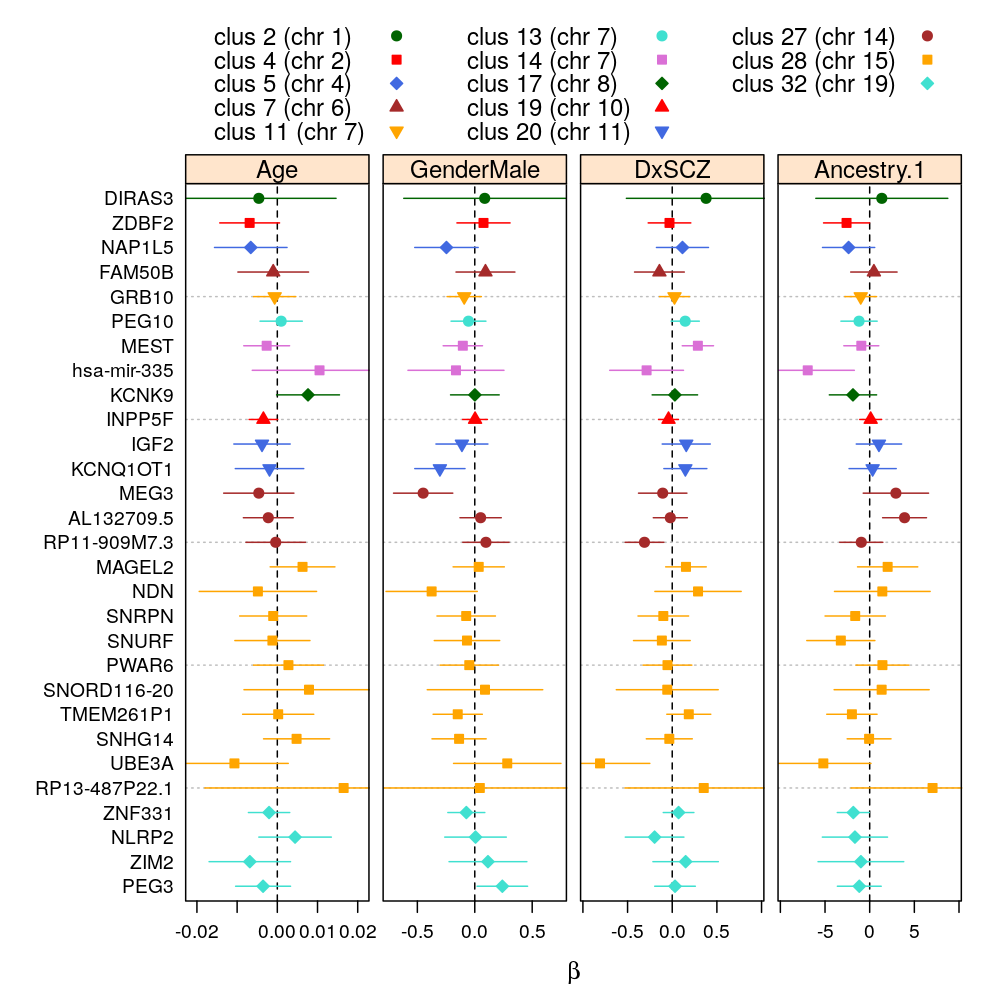
The main question queries the mechanism of the age effect on imprinting (loss, gain or lack of effect). In particular: does age regulate genes within some cluster in a concerted or an independent manner?
The current work studies this by performing two main steps
- delineation of clusters
- visualize clusters and age effect in terms of regression coefficients for age
Note that a table comparing imprinted genes identified by Baran et al to those by this study is available at baran-vs-ourwork.csv.
Data import and preparation
## Loading required package: RColorBrewer
Load data importer functions:
source("../../src/import-data.R")
source("../../src/utils.R")
source("~/projects/monoallelic-brain/src/fit-glms.R")
source("2016-08-08-imprinted-gene-clusters.R")
Genome-wide data
gene.summary <-
    read.csv("../../data/readcount/summary-all-genes.csv")
rownames(gene.summary) <- gene.summary$Symbol
gene.summary$file.size <-
    read.csv("../../data/readcount/fsize-genes.csv", row.names = 2)[rownames(gene.summary), , drop = TRUE]
gene.ids <- with(gene.summary, as.character(Symbol)[ file.size > 0 ])
genes2fit <- unlist(read.csv("../../data/genes.regression.new", as.is = TRUE))
names(genes2fit) <- genes2fit
Y <- get.readcounts(gene.ids, g.subsets = list(), sel.var = c("H", "N"), rm.conflict = TRUE)
S <- data.frame(lapply(gene.ids, function(g) Y[[g]]$H / Y[[g]]$N), check.names = FALSE)
names(S) <- gene.ids
N <- data.frame(lapply(Y, getElement, "N"), check.names = FALSE)
rm(Y)
Filtering
- read count-based filter with threshold
- individual-based filter with threshold
The code was copied from an earlier post and is hidden here.
Fitting models to selected genes
Import read count data but do not filter, to be consistent with the most recent regression analysis:
genes2fit <- unlist(read.csv("../../data/genes.regression.new", as.is = TRUE))
names(genes2fit) <- genes2fit
E <- get.predictors() # default arguments
Y <- get.readcounts(gene.ids = genes2fit, count.thrs = 0)
Fitting all models to all retained gene-wise and aggregated read count data sets
# exclude unweighed aggregates UA.8 and UA from fitting
ids2fit <- grep("^UA(.8)?$", names(Y), value = TRUE, invert = TRUE)
M <- do.all.fits(Y[ids2fit], preds = e.vars)
f.ids <- as.data.frame(lapply(M, function(m) ! sapply(m, is.null)))
f.ids["TMEM261P1", c("logi.S", "logi2.S")] <- FALSE
f.ids[c("WA.8", "WA"), ] <- FALSE # gene aggregates are not needed here
Analysis
Delineation of imprinted gene clusters
Let denote the set of genes such that means the gene is either “known” (to be imprinted) or near some “known”, i.e. “nearby candidate”. Let be the set of “candidate” genes (further away from “known”s). Let and be neighboring genes on the same chromosome at the -th and -th site. Delineation of clusters was done using the following simple rule: if and then a cluster starts at the -th gene. The cluster ends at the first such that but . The rule is implemented in the make.impr.segs function in 2016-08-08-imprinted-gene-clusters.R.
gene.summary$imprinting.status <- factor(gene.summary$imprinted, ordered = TRUE)
levels(gene.summary$imprinting.status) <- rev(c("known imprinted", "nearby candidate", "distant candidate"))
gene.summary$Symbol <- factor(gene.summary$Symbol, levels = gene.summary$Symbol, ordered = TRUE)
gene.summary$chr <- factor(paste("chr", gene.summary$chr), levels = paste("chr", seq_along(levels(factor(gene.summary$chr)))), ordered = TRUE)
# imprinting segments in component 'seg': clusters and segments inbetween
gs.seg <- make.impr.segs(gene.summary, remove.str = "distant candidate")
gs.seg$cluster <-
    factor(x <- with(gs.seg,
                     ifelse(seg > 0, paste0("clus ", seg, " (", chr, ")"), paste0("inter clus ", abs(seg)))),
           levels = unique(x), ordered = TRUE)
rm(x)
# remove filtered genes
gs <- gs.seg[names(frac), ]
gs$score <- unlist(frac["1", ])
Write results to file:
write.csv(gs, file = "../../results/gene-clusters.csv")
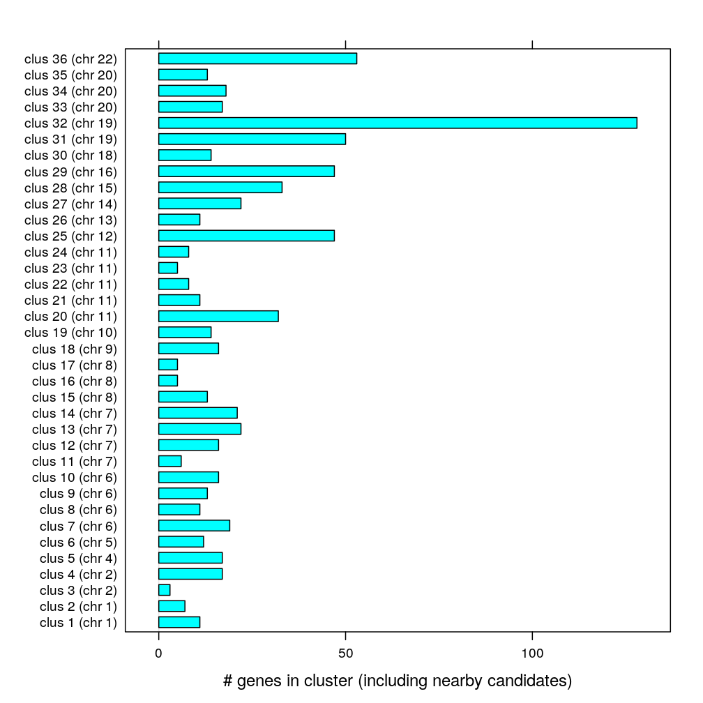
Eeach cluster has several genes including the “nearby candidate” category; note the median as well.
cluster.freq <- table(gs.seg$cluster)[seq(2, length(levels(gs.seg$cluster)), by = 2)]
median(cluster.freq)
## [1] 15
barchart(cluster.freq, xlab = "# genes in cluster (including nearby candidates)")
Before filtering these clusters contain the following number of “known” and “nearby candidate” genes:
table(gene.summary$imprinting.status)
##
## distant candidate  nearby candidate   known imprinted
##             15265               701                60
After filtering:
table(gs$imprinting.status)
##
## distant candidate  nearby candidate   known imprinted
##              4981               266                36
Genomic location
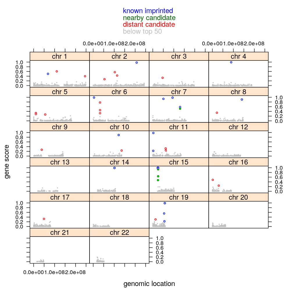
The plot below shows the genomic location of all 5283 genes in the filtered data set and indicates their imprinting status with different colors. Also shown is the gene score according to which genes have been ranked and called as monoallelically expressing or not.
gs$imprinting.status.1 <- as.character(gs$imprinting.status)
gs$imprinting.status.1[51:length(gs$imprinting.status.1)] <- "below top 50"
gs$imprinting.status.1 <- factor(gs$imprinting.status.1, levels = c("below top 50", levels(gs$imprinting.status)))
mycol <- c("gray", "red", "darkgreen", "blue")
xyplot(score ~ start | chr, data = gs, groups = imprinting.status.1,
       auto.key = list(text = rev(levels(gs$imprinting.status.1)), columns = 1, col = rev(mycol), points = FALSE),
       layout = c(4, 6),
       par.settings = list(superpose.symbol =
                           list(pch = c(21, 21, 21, 21), alpha = c(1, 1, 1, 1),
                                fill = c("white", "pink", "green", "lightblue"),
                                cex = c(0.2, 0.5, 0.5, 0.5),
                                col = mycol)),
       xlab = "genomic location", ylab = "gene score")
Extract and confidence intervals for
sel.genes <- unlist(read.csv("../../data/genes.regression.new", as.is = TRUE))
beta.99 <- lapply(M, function(l.m) do.beta(l.m[sel.genes], conf.lev = 0.99))
beta.95 <- lapply(M, function(l.m) do.beta(l.m[sel.genes], conf.lev = 0.95))
beta.99.long <- do.call(rbind, lapply(names(beta.99), function(x) cbind(beta.99[[x]], data.frame(Model = x))))
#write.csv(beta.99.long, "../../results/beta-99-CI.csv")
beta.95.long <- do.call(rbind, lapply(names(beta.99), function(x) cbind(beta.99[[x]], data.frame(Model = x))))
#write.csv(beta.95.long, "../../results/beta-95-CI.csv")
Filtering for poor fit
Filter based on earlier decisions on the goodness of fit of logi.S, which is stored in results/model-checking.csv.
logi.S.OK <- read.csv("../../results/model-checking.csv", row.names = "gene")["logi.S.fit.OK"]
# set results to NA where logi.S fitted poorly
beta.99$logi.S[beta.99$logi.S$Gene %in% rownames(logi.S.OK)[! logi.S.OK$logi.S.fit.OK],
               c("Estimate", "Lower.CL", "Upper.CL")] <- NA
beta.95$logi.S[beta.95$logi.S$Gene %in% rownames(logi.S.OK)[! logi.S.OK$logi.S.fit.OK],
               c("Estimate", "Lower.CL", "Upper.CL")] <- NA
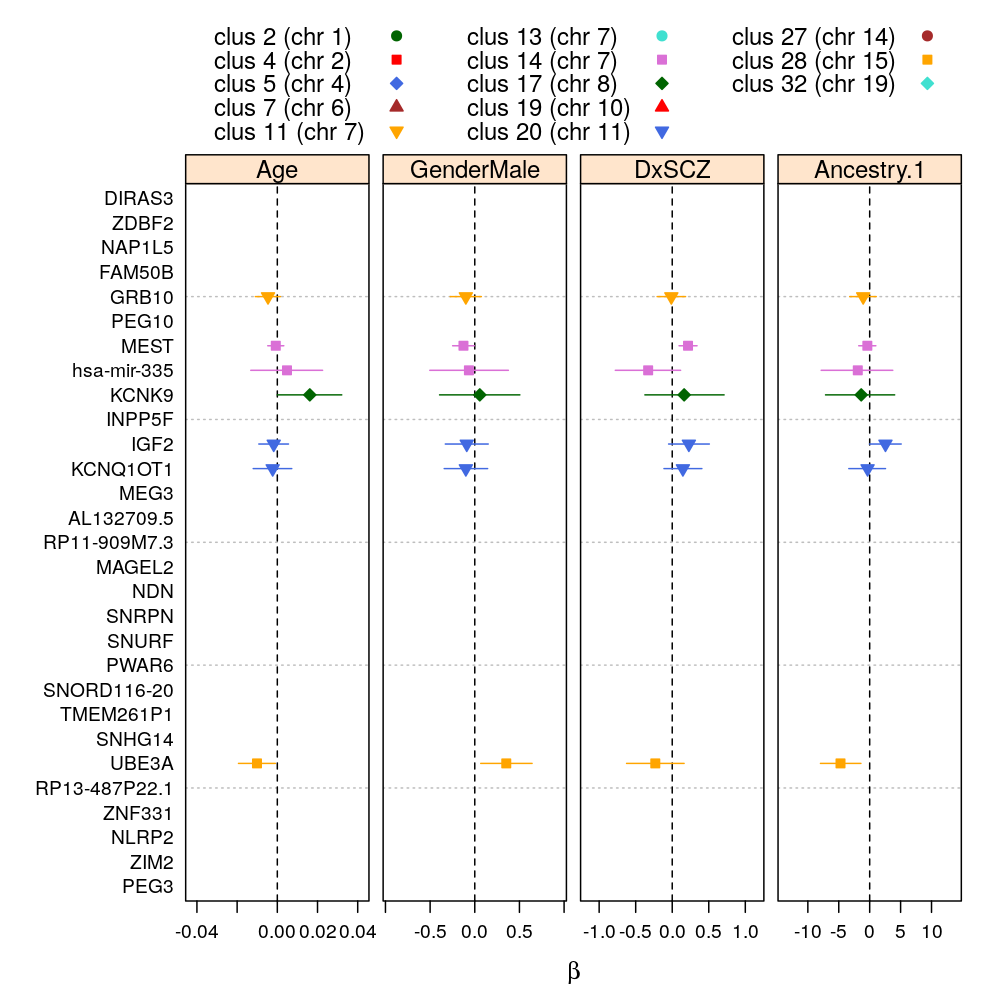
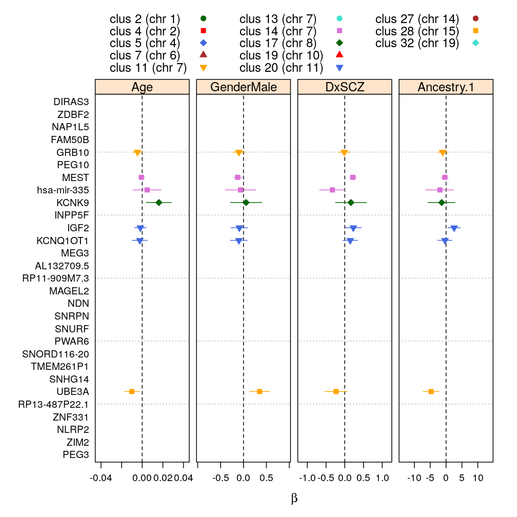
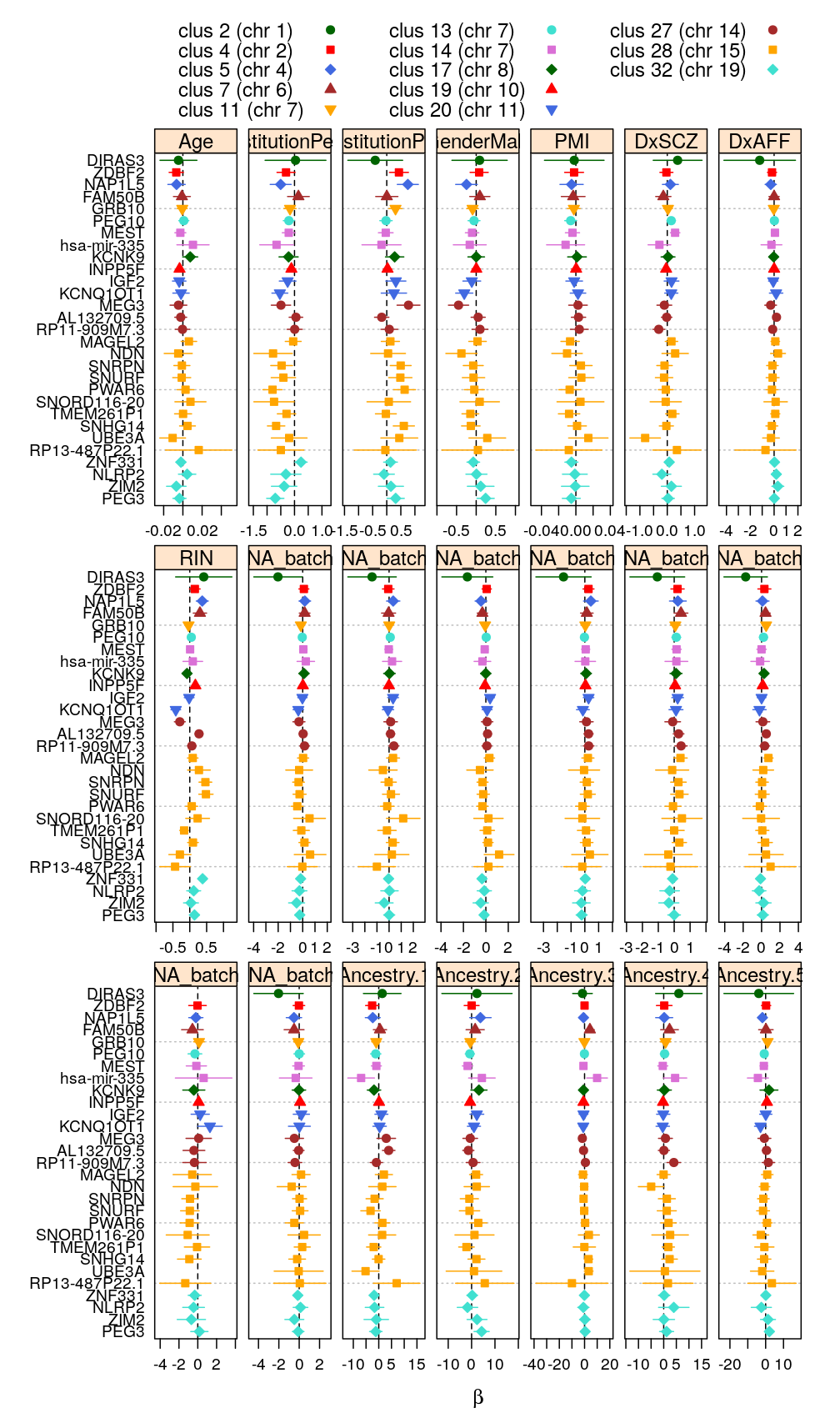
arranged by clusters
wnlm.Q, 99 % confidence (for the manuscript)
my.segplot2(beta.99$wnlm.Q, layout = c(4, 1), xlim = list(2e-2*c(-1,1), 0.7*c(-1,1), 0.9*c(-1,1), 9*c(-1,1)))
wnlm.Q, 95 % confidence

logi.S, 99 % confidence
logi.S, 95 % confidence
my.segplot2(beta.99$wnlm.Q, layout = c(7, 3), sel.coefs = unlist(lapply(e.vars, function(v) predictor2coefs(M$wnlm.Q[[1]], v))))
Comparison to Baran et al 2015
Baran et al 2015 identified 42 imprinted genes in various human tissues based on GTeX and other data. Their Table S3 lists these genes along with the tissue in which they were found to be imprinted:
baran <- read.csv("../../data/baran-2015-genome-res/table_s3.csv")
levels(baran$name)
##  [1] "CPA4"        "CST1"        "DIRAS3"      "DLK1"        "FAM50B"
##  [6] "GRB10"       "H19"         "IGF2"        "IGF2-AS"     "INPP5F_V2"
## [11] "KCNQ1"       "KIF25"       "L3MBTL1"     "LPAR6"       "MAGEL2"
## [16] "MAGI2"       "MEG3"        "MEG8"        "MEG9"        "MEST"
## [21] "MKRN3"       "NAP1L5"      "NDN"         "NTM"         "PEG10"
## [26] "PEG3"        "PLAGL1"      "PPIEL"       "PRSS50"      "PWRN1"
## [31] "RP11-7F17.7" "SNHG14"      "SNRPN"       "SNURF"       "SYCE1"
## [36] "THEGL"       "UBE3A"       "UGT2B4"      "UTS2"        "ZDBF2"
## [41] "ZNF331"      "ZNF597"
Establish consistency of gene names between Baran et al and our study and extract genes Baran et al found to be imprinted in the brain:
levels(baran) <- sub("INPP5F_V2", "INPP5F", levels(baran$name))
levels(baran) <- sub("MEG8", "RP11-909M7.3", levels(baran$name))
baran$name <- sub("INPP5F_V2", "INPP5F", baran$name)
baran$name <- sub("MEG8", "RP11-909M7.3", baran$name)
baran.brain <- baran[ baran$tissue == "BRAIN", "name"]
Summarize genes called imprinted either by Baran et al or this study:
##                            this.work
## Baran.et.al                 imprinted not imprinted not assessed
##   imprinted                        19            12            9
##   not imprinted or assessed        10             0            0
Next, list each gene and write result to file. It is noteworthy that the novel imprinted genes suggested by our study are RP11-909M7.3, TMEM261P1, AL132709.5, PWAR6, SNORD116-20, RP13-487P22.1, hsa-mir-335 and among these only RP11-909M7.3 is/are suggested by Baran et al.
baran.vs.ourwork[ , -1]
##                             Baran.et.al     this.work    prior.status
## CPA4                          imprinted  not assessed            <NA>
## DIRAS3                        imprinted     imprinted known_imprinted
## DLK1                          imprinted  not assessed            <NA>
## FAM50B                        imprinted     imprinted known_imprinted
## GRB10                         imprinted     imprinted known_imprinted
## H19                           imprinted not imprinted known_imprinted
## IGF2                          imprinted     imprinted known_imprinted
## IGF2-AS                       imprinted  not assessed            <NA>
## INPP5F                        imprinted     imprinted known_imprinted
## KCNQ1                         imprinted  not assessed known_imprinted
## KIF25                         imprinted not imprinted               _
## L3MBTL1                       imprinted not imprinted  1 M impr clstr
## LPAR6                         imprinted not imprinted  1 M impr clstr
## MAGEL2                        imprinted     imprinted known_imprinted
## MAGI2                         imprinted not imprinted known_imprinted
## MEG3                          imprinted     imprinted known_imprinted
## RP11-909M7.3                  imprinted     imprinted  1 M impr clstr
## MEG9                          imprinted not imprinted known_imprinted
## MEST                          imprinted     imprinted known_imprinted
## MKRN3                         imprinted not imprinted known_imprinted
## NAP1L5                        imprinted     imprinted known_imprinted
## NDN                           imprinted     imprinted known_imprinted
## NTM                           imprinted not imprinted known_imprinted
## PEG10                         imprinted     imprinted known_imprinted
## PEG3                          imprinted     imprinted known_imprinted
## PLAGL1                        imprinted not imprinted known_imprinted
## PPIEL                         imprinted  not assessed            <NA>
## PRSS50                        imprinted  not assessed            <NA>
## PWRN1                         imprinted not imprinted  1 M impr clstr
## RP11-7F17.7                   imprinted  not assessed            <NA>
## SNHG14                        imprinted     imprinted known_imprinted
## SNRPN                         imprinted     imprinted known_imprinted
## SNURF                         imprinted     imprinted known_imprinted
## SYCE1                         imprinted not imprinted               _
## THEGL                         imprinted  not assessed            <NA>
## UBE3A                         imprinted     imprinted known_imprinted
## UTS2                          imprinted  not assessed            <NA>
## ZDBF2                         imprinted     imprinted known_imprinted
## ZNF331                        imprinted     imprinted known_imprinted
## ZNF597                        imprinted not imprinted known_imprinted
## TMEM261P1     not imprinted or assessed     imprinted  1 M impr clstr
## AL132709.5    not imprinted or assessed     imprinted  1 M impr clstr
## ZIM2          not imprinted or assessed     imprinted known_imprinted
## PWAR6         not imprinted or assessed     imprinted  1 M impr clstr
## KCNQ1OT1      not imprinted or assessed     imprinted known_imprinted
## SNORD116-20   not imprinted or assessed     imprinted  1 M impr clstr
## KCNK9         not imprinted or assessed     imprinted known_imprinted
## RP13-487P22.1 not imprinted or assessed     imprinted  1 M impr clstr
## hsa-mir-335   not imprinted or assessed     imprinted  1 M impr clstr
## NLRP2         not imprinted or assessed     imprinted known_imprinted
write.csv(baran.vs.ourwork, file = "../../results/baran-vs-ourwork.csv", row.names = FALSE)
Revision for Nature Communications
This part is motivated by the following comments from reviewer #2
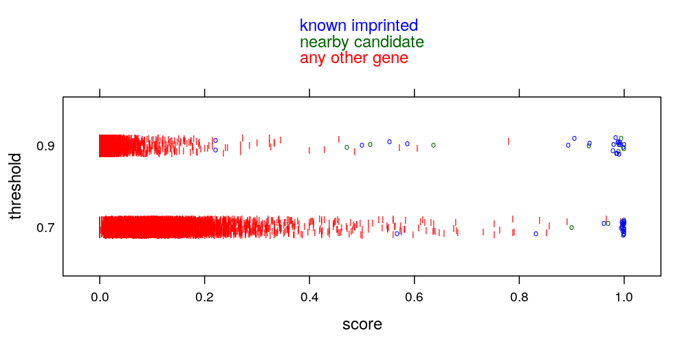
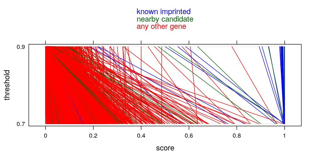
How robust the results are the arbitrarily chosen “S_{ig} > 0.9” threshold? If 0.7 were chosen how would the top 50 genes change? Couldn’t genes simply be ranked by the sum of the S_{ig} scores across individuals? Similar question about the “top 50” genes, why 50, how would the top 20, top 100 behave in terms of imprinting enrichment? Wouldn’t it be simpler to make the point by drawing a ROC curve (truth=known imprinted genes, S_{ig}>.9 fraction as predictor)?
gs.0.9 <- cbind(gs, data.frame(ecdf.thrs = factor("0.9")))
gs.0.7 <- cbind(gs, data.frame(ecdf.thrs = factor("0.7")))
gs$score.0.7 <- gs.0.7$score <- apply(frac[1:3, ], 2, sum)
gs.long <- rbind(gs.0.7, gs.0.9)
rm(gs.0.9, gs.0.7)
mykey <- list(text = c(rev(levels(gs$imprinting.status.1)[-1:-2]), "any other gene"), columns = 1, col = rev(mycol[-1]), points = FALSE, lines = FALSE)
mypar <- list(superpose.line = list(col = c(mycol[-1])), superpose.symbol = list(col = c("red", mycol[-1])))
parallelplot(gs[c("score.0.7", "score")], groups = gs$imprinting.status,
       par.settings = mypar, auto.key = mykey, ylab = "threshold", xlab = "score",
       scales = list(x = list(at = seq(from = 0, to = 1, by = 0.2), labels = as.character(seq(from = 0, to = 1, by = 0.2))),
                     y = list(at = 1:2, labels = c("0.7", "0.9"))))
stripplot(ecdf.thrs ~ score, data = gs.long, groups = imprinting.status.1, jitter = TRUE,
       par.settings = mypar, ylab = "threshold",
       auto.key = mykey, pch = c("I", "I", "o", "o"))
