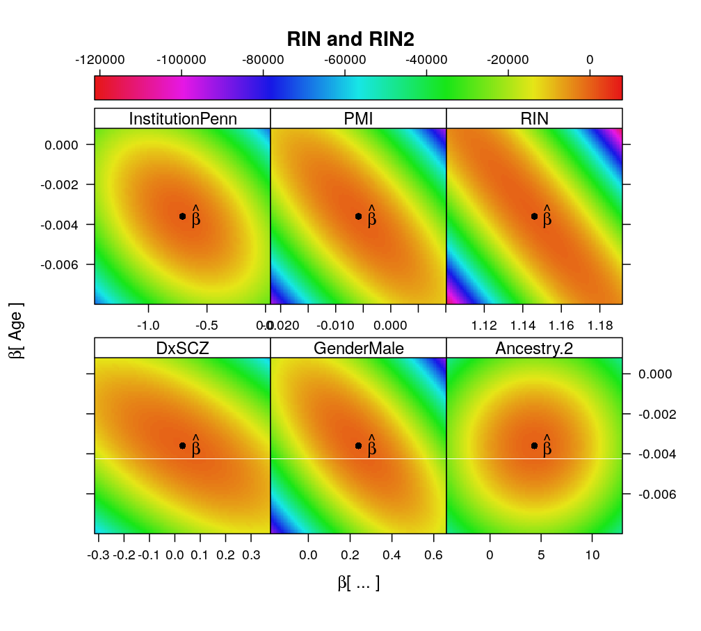
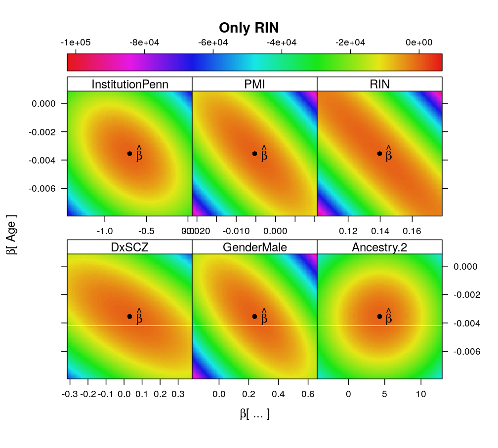
Some shortcomings of the previous design matrix are inspected and corrected here. These include highly collinear terms as well as awkward allocation of control and treatment factors.
Motivation
Previous analysis used a design matrix with the following shortcomings
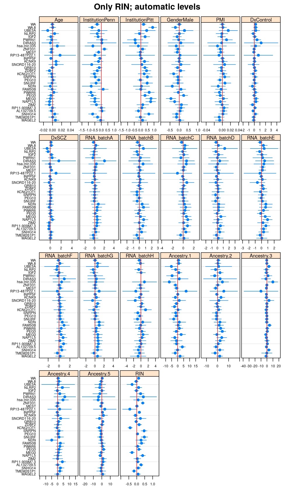
- the baseline level of certain factors in was automatically set; in particular for Dx the baseline level was AFF instead of Control
- contained a pair of nearly collinear predictors RIN and RIN2 (squared)
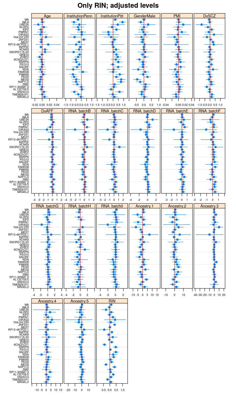
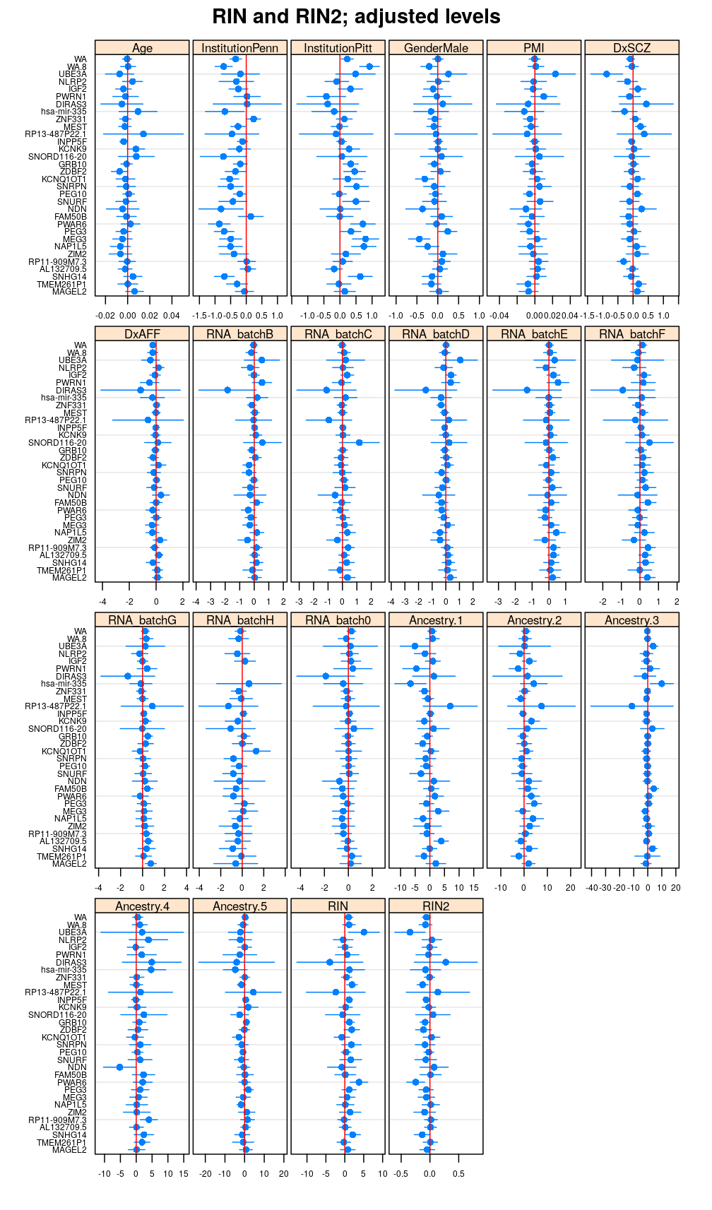
These shortcomings are corrected here and the corresponding changes in results are studied. The results show that the corrections afford minor improvements:
- SCZ is now directly contrasted to Control, revealing significant effect for some genes
- with the removal of RIN2 the term associated with RIN is no more much larger than those with other predictors
Results
Preliminaries
## Loading required package: RColorBrewer
##
## Attaching package: 'latticeExtra'
## The following object is masked from 'package:ggplot2':
##
##     layer
source("../../src/import-data.R")
source("../../src/fit-glms.R")
source("../../src/likelihood-surface.R")
source("../../src/graphics.R")
# explanatory variables (a.k.a. predictors)
e.vars2 <- c("Age",
               "Institution",
               "Gender",
               "PMI",
               "Dx",
               "RIN",
               "RIN2", # to be removed
               "RNA_batch",
               "Ancestry.1", "Ancestry.2", "Ancestry.3", "Ancestry.4", "Ancestry.5" )
e.vars <- e.vars2[-7] # removing RIN2
E <- get.predictors() # default arguments
E.al <- get.predictors(adj.levels = FALSE) # automatic (unadjusted) levels
Y <- get.readcounts(gene.ids = gene.ids, count.thrs = 0)
to.fit.ids <- grep("^UA(.8)?$", names(Y), value = TRUE, invert = TRUE) # exclude unweighed aggregates UA.8 and UA from fitting
sel.models <- c("logi.S", "wnlm.Q", "wnlm.R", "unlm.Q"); names(sel.models) <- sel.models
M <- do.all.fits(Y[to.fit.ids], G = E, preds = e.vars, sel.models = sel.models)
M.al <- do.all.fits(Y[to.fit.ids], G = E.al, preds = e.vars, sel.models = sel.models)
M2 <- do.all.fits(Y[to.fit.ids], G = E, preds = e.vars2, sel.models = sel.models)
Estimates and CIs
Betas <- lapply(M, function(m) { x <- get.estimate.CI(m); x <- x[ ! x$Coefficient %in% "(Intercept)", ] })
Betas.al <- lapply(M.al, function(m) { x <- get.estimate.CI(m); x <- x[ ! x$Coefficient %in% "(Intercept)", ] })
Betas2 <- lapply(M2, function(m) { x <- get.estimate.CI(m); x <- x[ ! x$Coefficient %in% "(Intercept)", ] })
Terms
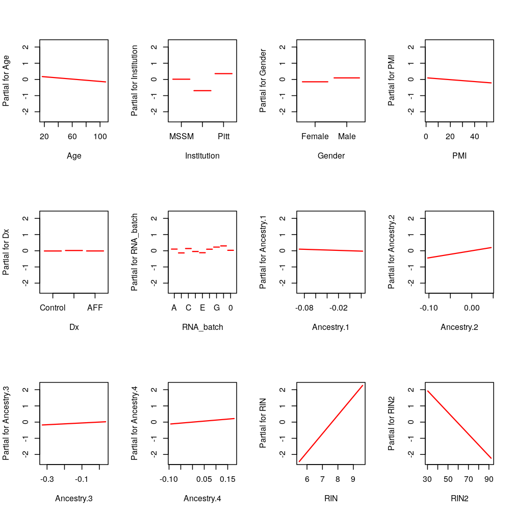
PEG3: RIN and RIN2
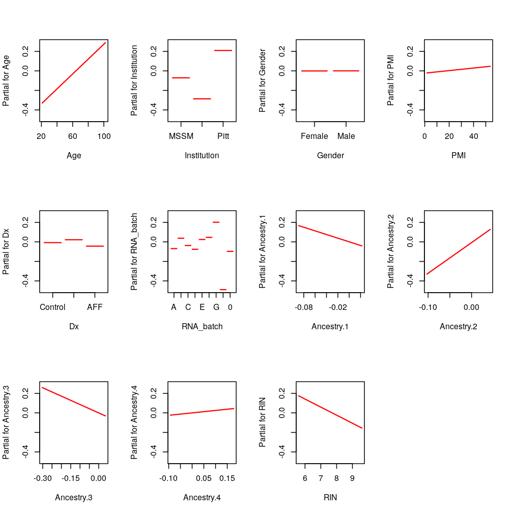
par(mfrow = c(3, 4))
termplot(M2$wnlm.Q$PEG3, terms = c(1:5, 8:12, 6:7))
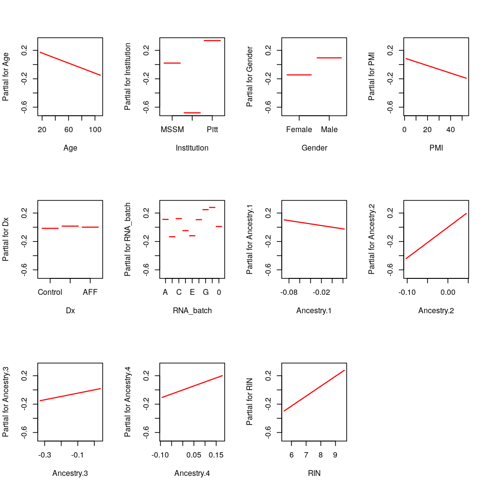
PEG3: only RIN
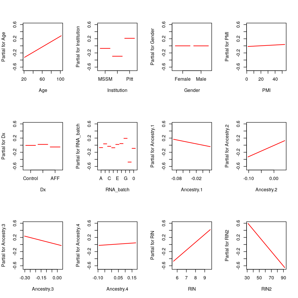
KCNK9: RIN and RIN2
KCNK9: only RIN
Likelihood surface
