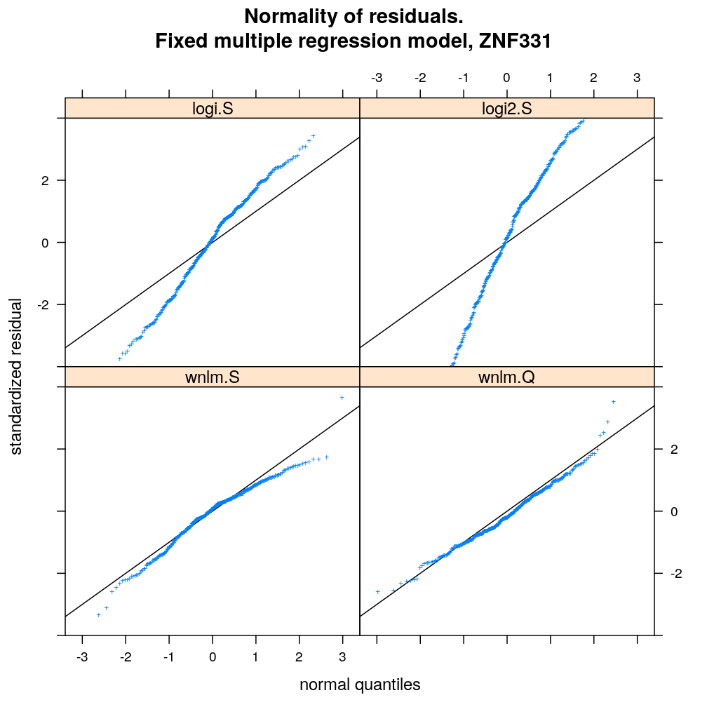
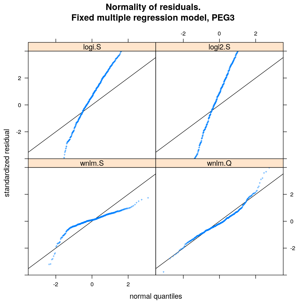
For a fixed set of terms in the linear predictor and for each gene, different data transformations, link functions, and error distributions are compared in terms of model fit. Fit is evaluated by diagnostic plots by inspecting the normality of residuals and the homogeneity of error (homoscedasticity). Although model fit varies across genes, taken all genes together the wnlm.Q and unlm.Q models emerge as the best fitting ones.
Click model-checking.csv to download the saved csv files reporting which genes were excluded under the logi.S model.
## Loading required package: RColorBrewer
##
## Attaching package: 'latticeExtra'
## The following object is masked from 'package:ggplot2':
##
##     layer
Preliminaries
Load functions
source("~/projects/monoallelic-brain/src/import-data.R")
source("~/projects/monoallelic-brain/src/fit-glms.R")
source("2016-09-23-model-checking.R")
gene.ids <- unlist(read.csv("../../data/genes.regression.new", as.is = TRUE))
names(gene.ids) <- gene.ids
Get data
E <- get.predictors() # default arguments
Y <- get.readcounts(gene.ids = gene.ids, count.thrs = 0)
Checking known outliers
Import outliers of the CMC study provided by Mette and Jessica and check if any has been included in our previous analyses. The answer is: they have all been excluded.
read.csv("../../data/outliers.csv", colClasses = "character")$DissectionID %in% row.names(E)
##  [1] FALSE FALSE FALSE FALSE FALSE FALSE FALSE FALSE FALSE FALSE FALSE
## [12] FALSE
Evaluation of model fit
Below is a visual evaluation of model fit using all 6 model types (unlm.S, wnlm.S, unlm.R, wnlm.R, logi.S, logi2.S) on each of the 30 data sets that represent the 30 selected genes for regression analysis. This visual evaluation is based on three kind of plots, which check the following aspects of model fit:
- normality of residuals
- homogieneity of error (homoscedasticity)
- influence of individual cases
These points will be detailed in the respective sections.
Start by fitting all models:
# exclude unweighed aggregates UA.8 and UA from fitting
to.fit.ids <- grep("^UA(.8)?$", names(Y), value = TRUE, invert = TRUE)
sel.models <- c("logi.S", "logi2.S", "unlm.Q", "wnlm.Q", "wnlm.R", "wnlm.S"); names(sel.models) <- sel.models
#sel.models <- NULL
M <- do.all.fits(Y[to.fit.ids], G = E, preds = e.vars, sel.models = sel.models)
Calculate diagnostics:
diagnostics <- lapply(names(M), function(m) get.diagnostics(M[[m]][gene.ids], mtype = m))
diagnostics <- do.call(rbind, diagnostics)
#diagnostics$gene <- factor(diagnostics$gene, levels = rev(levels(diagnostics$gene)), ordered = TRUE)
Normality of residuals
Two kind of standardized residual is plotted against the quantiles of the standard normal distribution:
- standardized deviance residual,
- a combination of the standardized deviance and Pearson residuals (the latter denoted as )
The combination is defined as in Statistical Models (A.C. Davison), p477: . Note that , and differ for generalized linear models such as logi.S and logi2.S but for linear models they all equal the usual definition of residual i.e. the observed minus fitted value .
skip <- ! sapply(M$logi.S, `[[`, "converged")[1:30]
myqqnorm <- function(mtype, skip = FALSE, ...)
    qqmath(~ res.std.dev + res.combined | gene, data = diagnostics,
           ylim = c(-4, 4), abline = c(0, 1), pch = "+", subset = model.type %in% mtype,
           par.settings = list(add.text = list(cex = 0.8)),
           skip = skip, layout = c(6, 5),
           main = mtype, xlab = "normal quantiles", ylab = "standardized residual",
           ...)[c(1:30)[! skip]]
#myqqnorm("unlm.S")
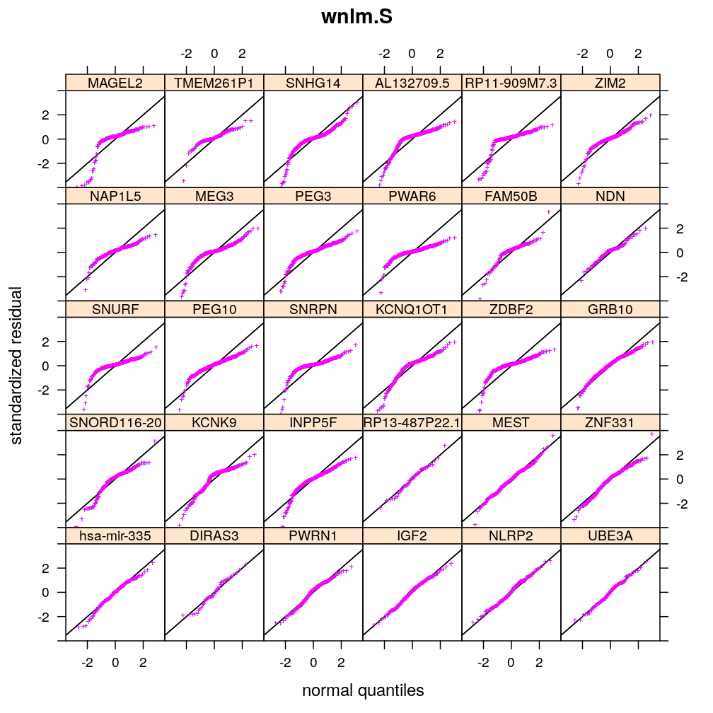
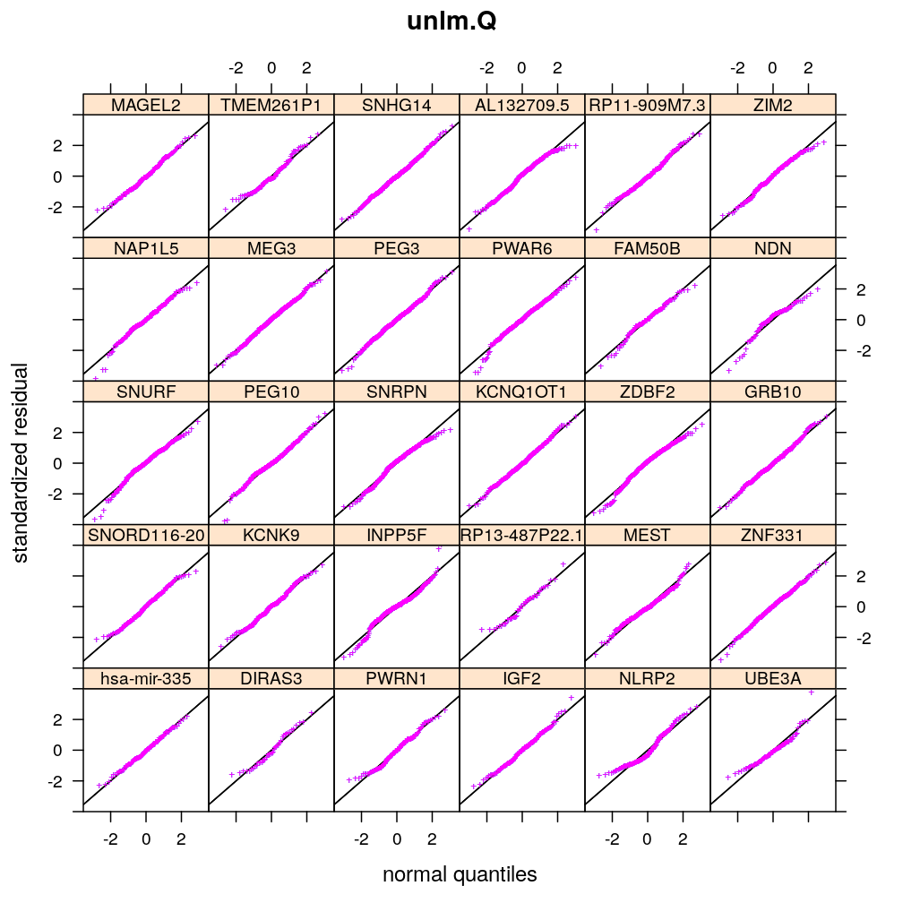
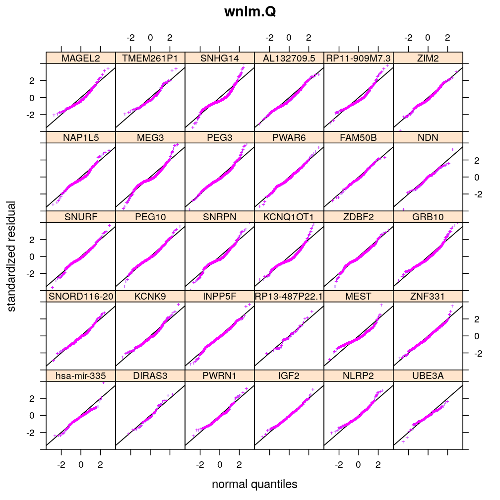
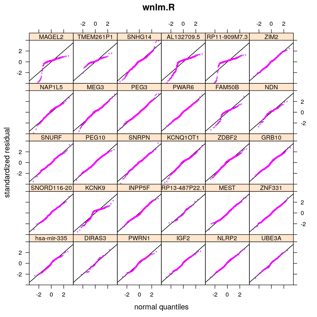
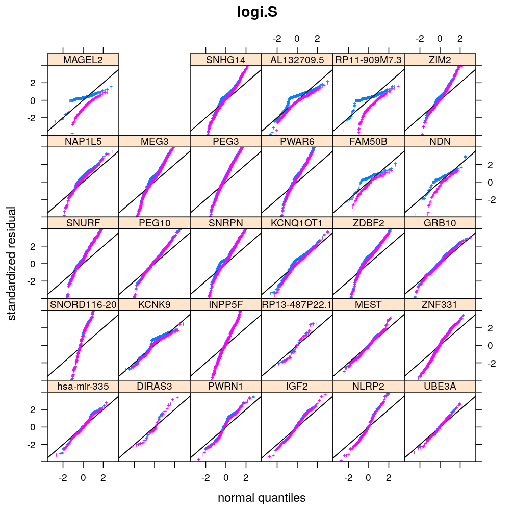
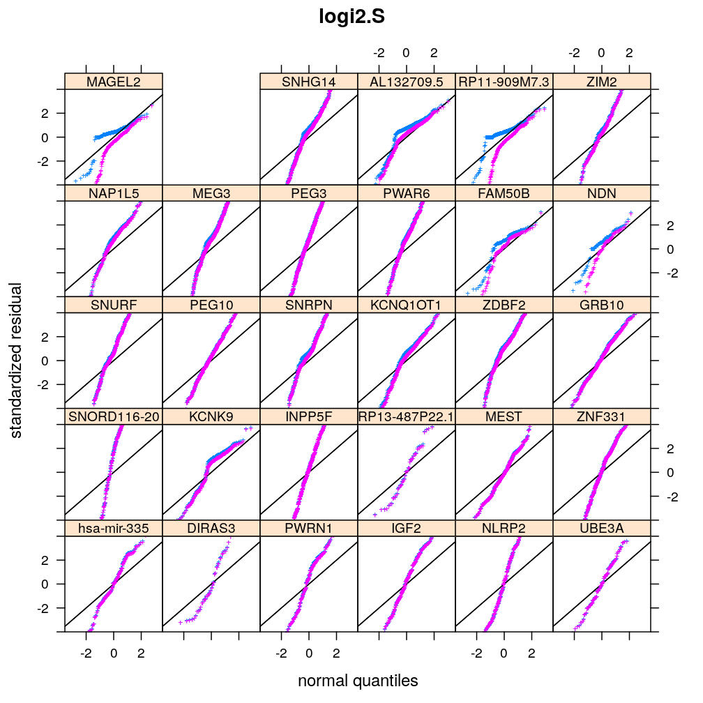
Figure for presentation
myqqnorm.demo <- function(g = "ZNF331") {
    qqmath(~ res.std.dev | model.type, data = diagnostics, subset = gene == g & model.type != "wnlm.R",
               ylim = c(-4, 4), abline = c(0, 1), pch = "+",
               main = paste("Normality of residuals.
Fixed multiple regression model,", g), xlab = "normal quantiles", ylab = "standardized residual",
           )[c(1:2, 5, 4)]
}
myqqnorm.demo("ZNF331")
myqqnorm.demo("PEG3")
myqqnorm.demo("ZDBF2")
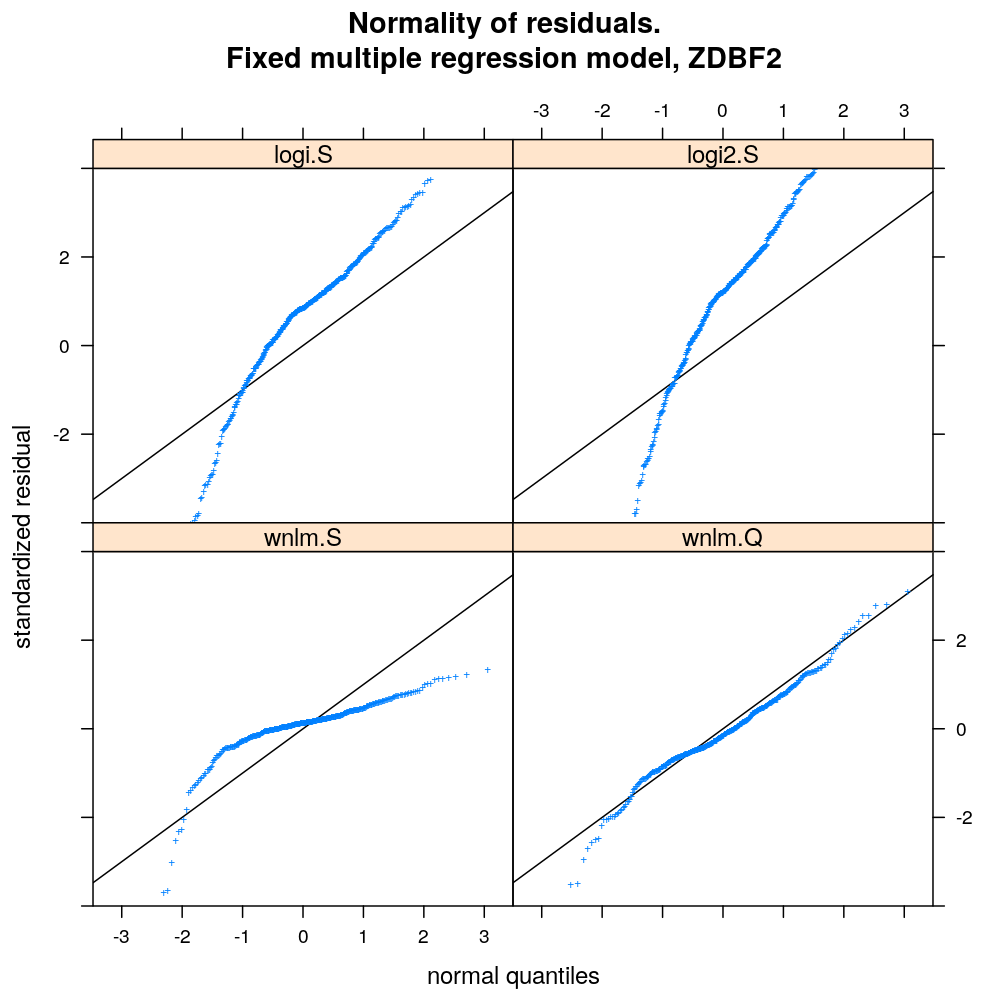
myqqnorm.demo("KCNK9")
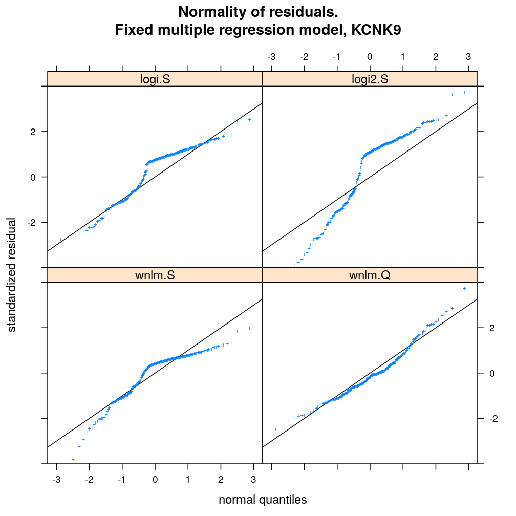
myqqnorm2(genes = c("MEST", "INPP5F"), models = c("wnlm.Q", "unlm.Q"))
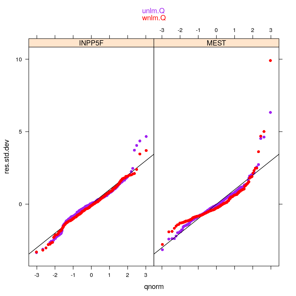
myqqnorm2(genes = gene.ids, models = c("wnlm.Q", "unlm.Q"))
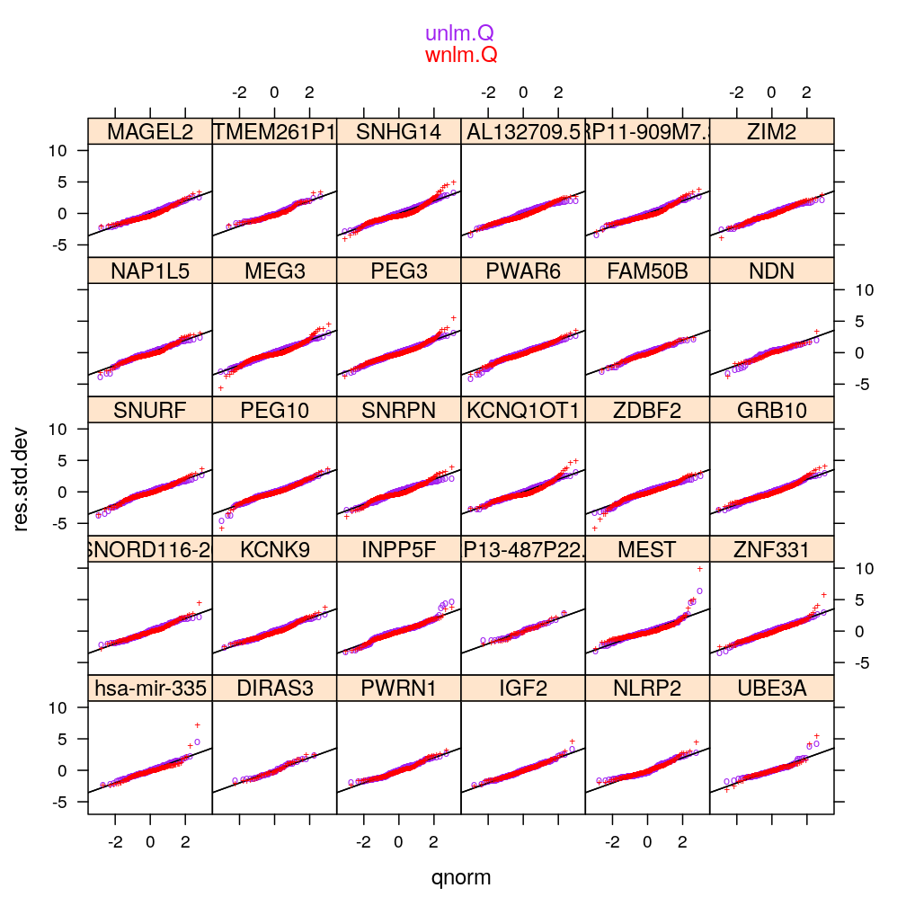
Homogeneity of error (homoscedasticity)
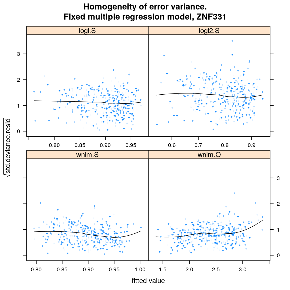
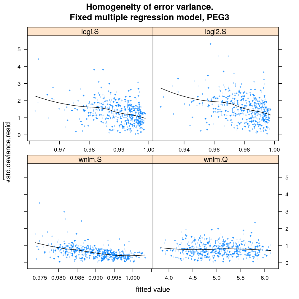
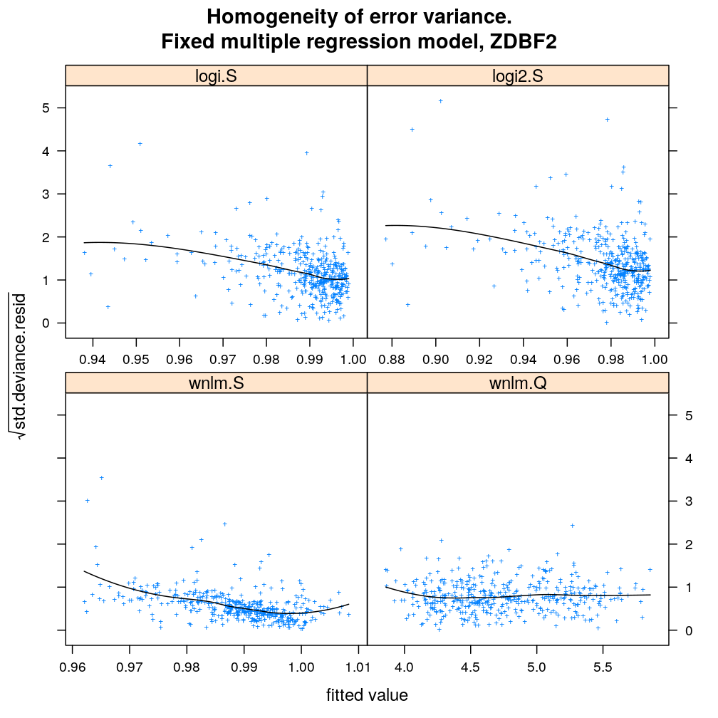
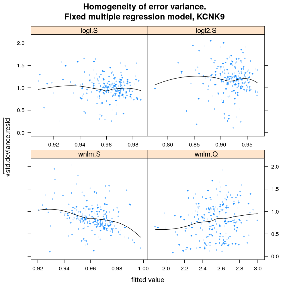
is plotted against the fitted value . The black lines correspond to the data passed through a LOESS filter. All models assume homogeneous error that is no systematic variation with the fitted value.
myhomoscedas <- function(mtype, skip = FALSE)
    xyplot(sqrt(abs(res.std.dev)) ~ fitted | gene, data = diagnostics,
           panel = function(...) {
               panel.xyplot(...)
               panel.smoother(..., method = "loess", col = "black", se = FALSE)
           },
           scales = list(x = list(relation = "free", draw = FALSE)),
           skip = skip, layout = c(6, 5),
           par.settings = list(add.text = list(cex = 0.8)),
           subset = model.type %in% mtype, pch = "+", main = mtype, xlab = "fitted value",
           ylab = expression(sqrt(std.deviance.resid)))[c(1:30)[! skip]]

#myhomoscedas("unlm.S")
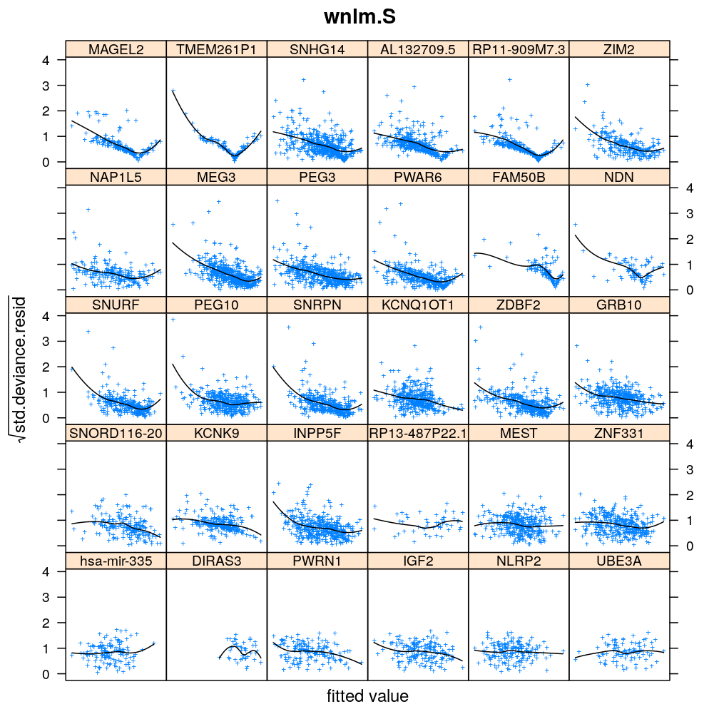
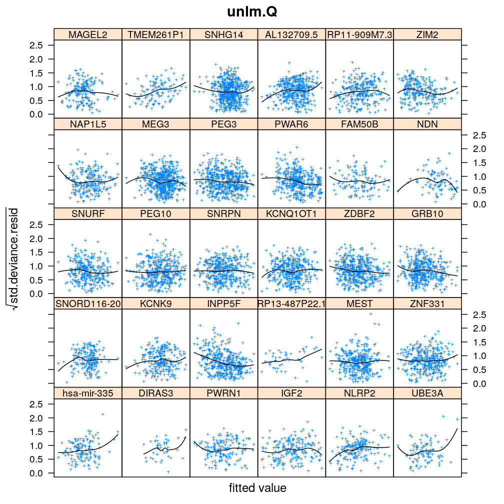
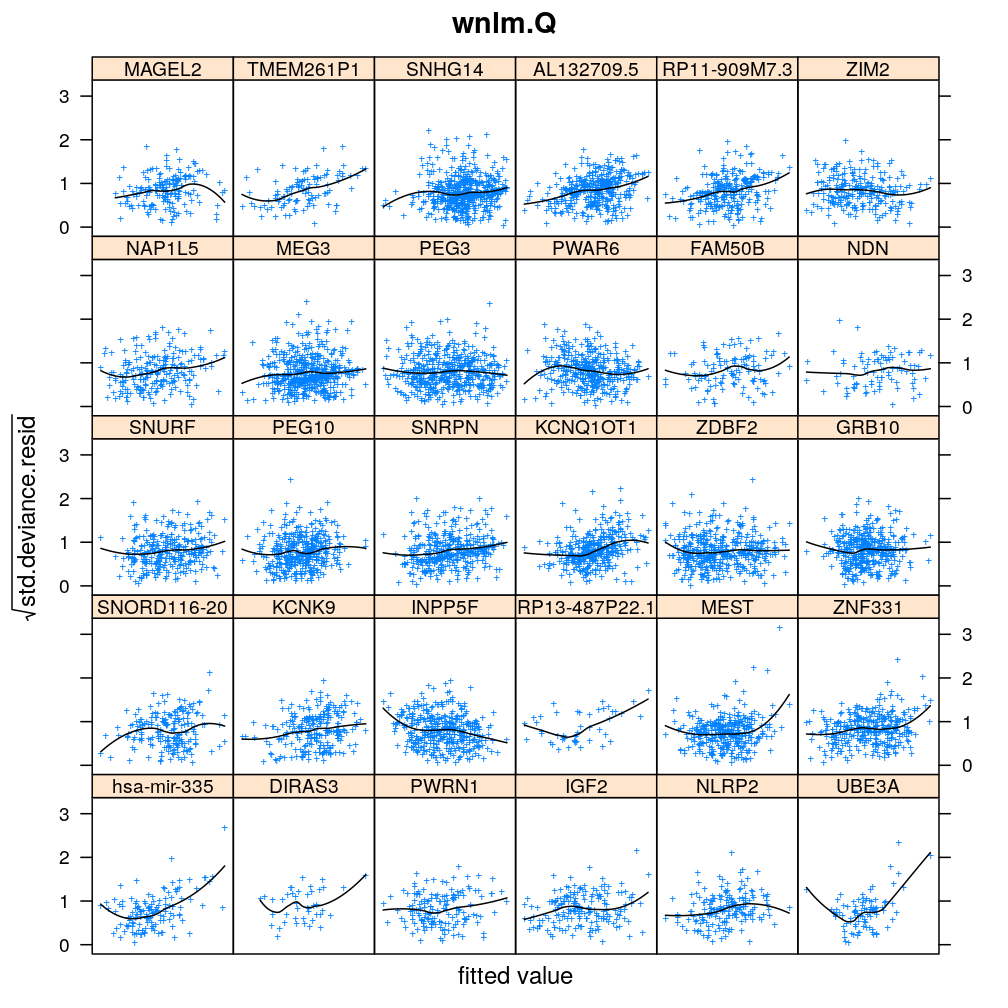
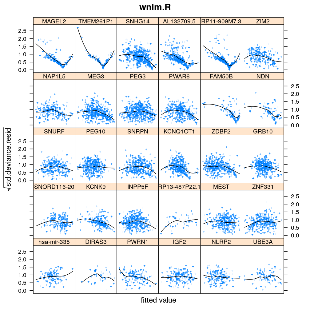
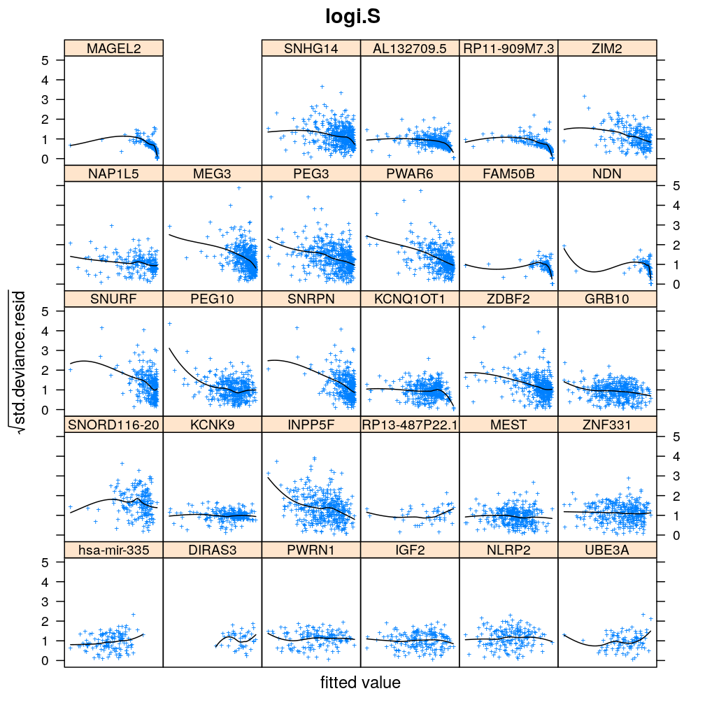
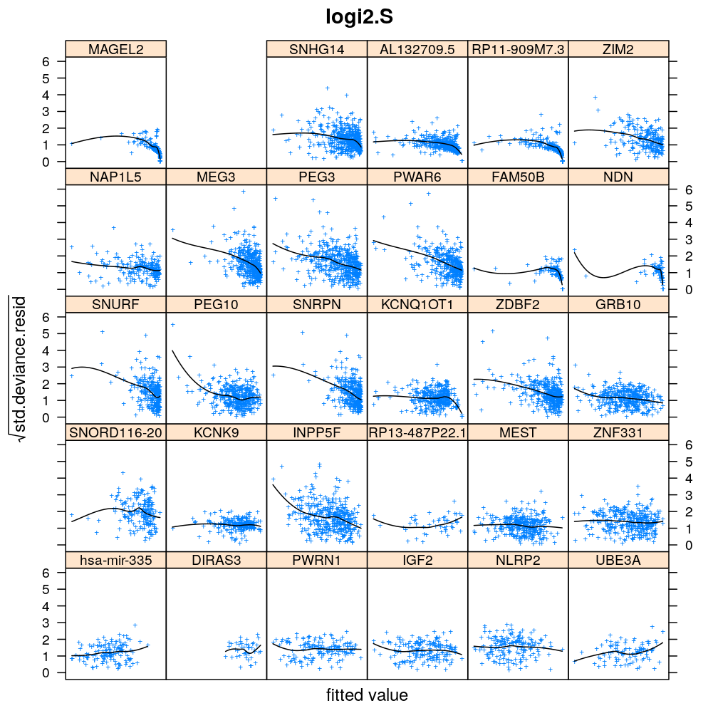
Figure for presentation
myhomoscedas.demo <- function(g) {
    xyplot(sqrt(abs(res.std.dev)) ~ fitted | model.type, data = diagnostics,
           panel = function(...) {
               panel.xyplot(...)
               panel.smoother(..., method = "loess", col = "black", se = FALSE)
           }, subset = gene == g & model.type != "wnlm.R", pch = "+",
           scales = list(x = list(relation = "free", draw = TRUE)),
           xlab = "fitted value", ylab = expression(sqrt(std.deviance.resid)),
           main = paste("Homogeneity of error variance.
Fixed multiple regression model,", g))[c(1:2, 5, 4)]
}
myhomoscedas.demo("ZNF331")
myhomoscedas.demo("PEG3")
myhomoscedas.demo("ZDBF2")
myhomoscedas.demo("KCNK9")
Influence of individual cases
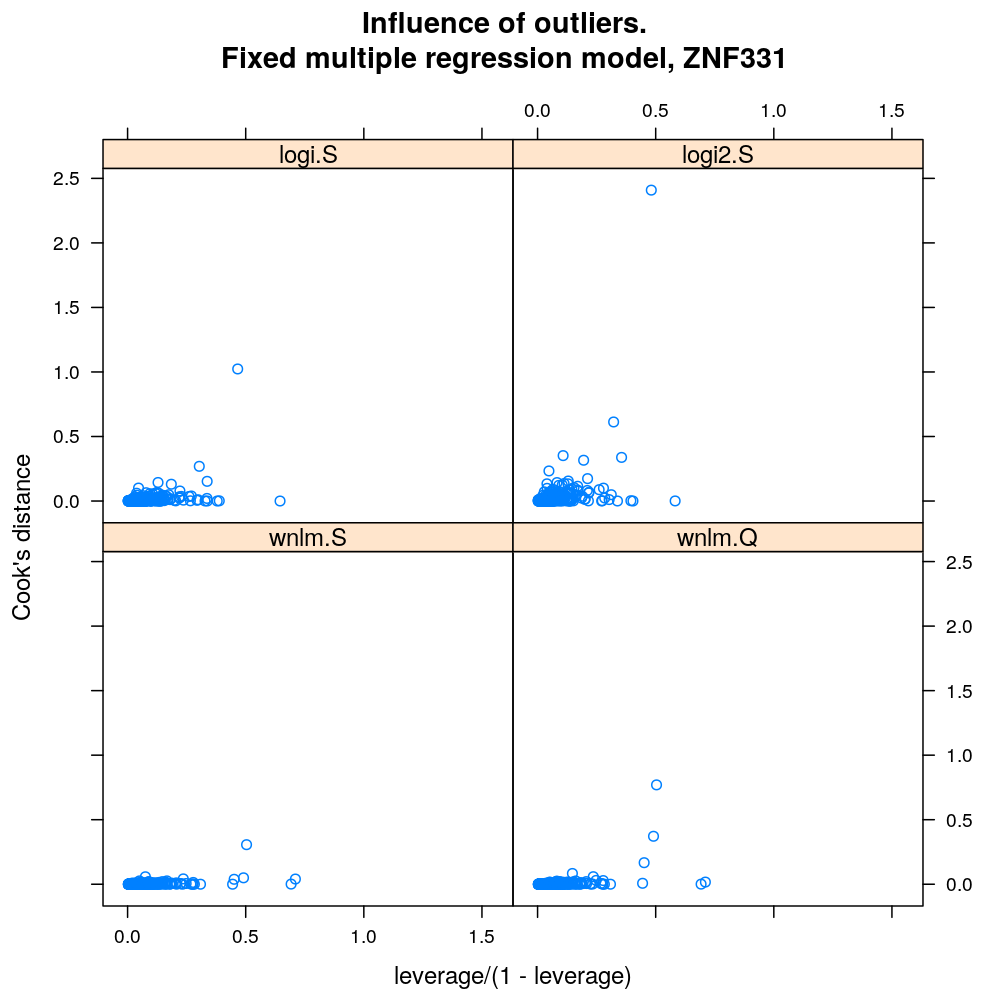
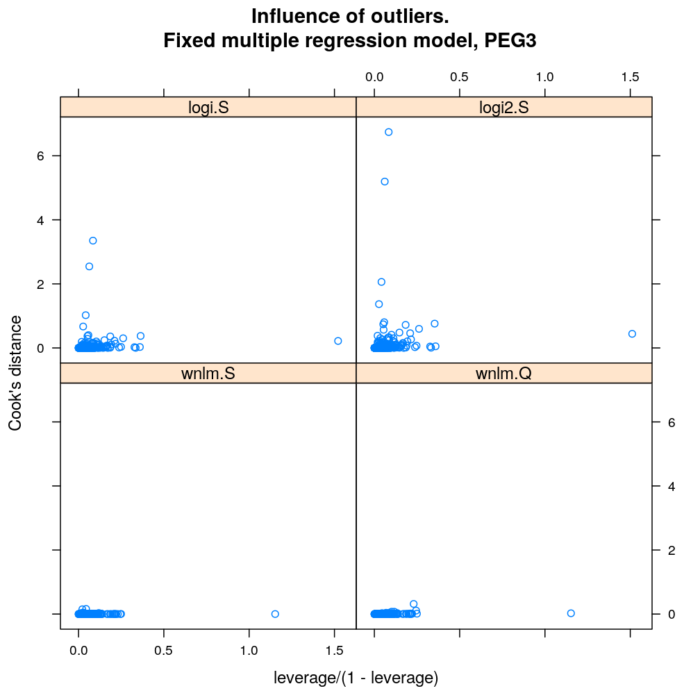
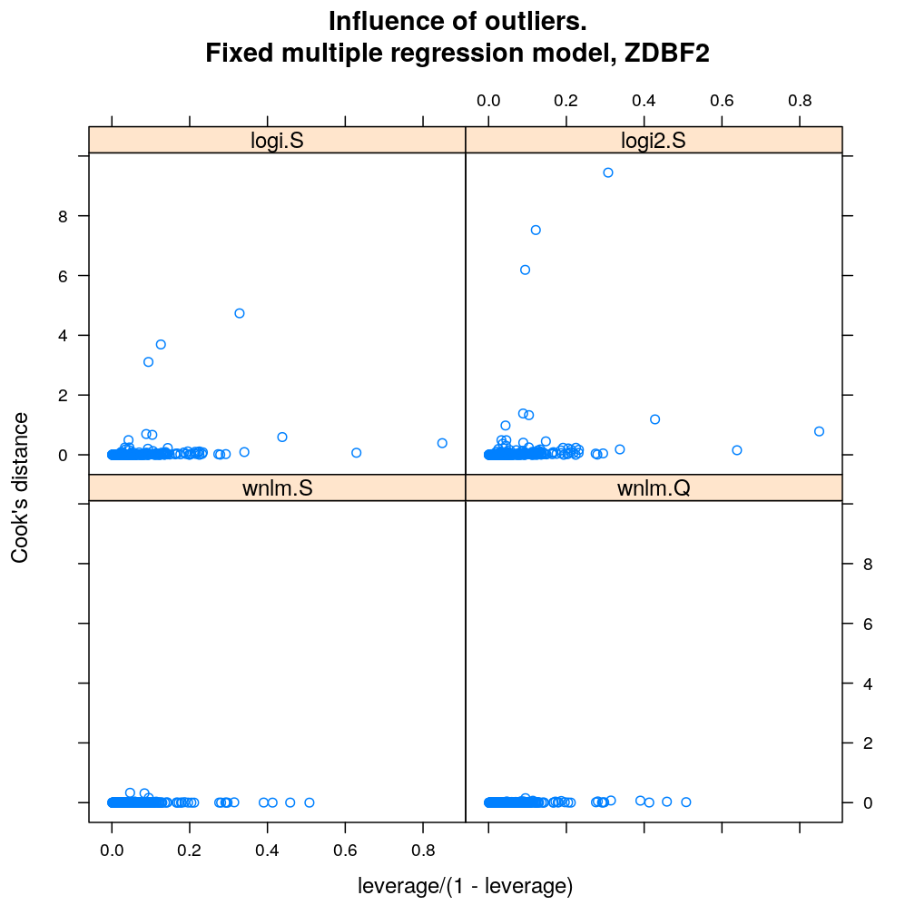
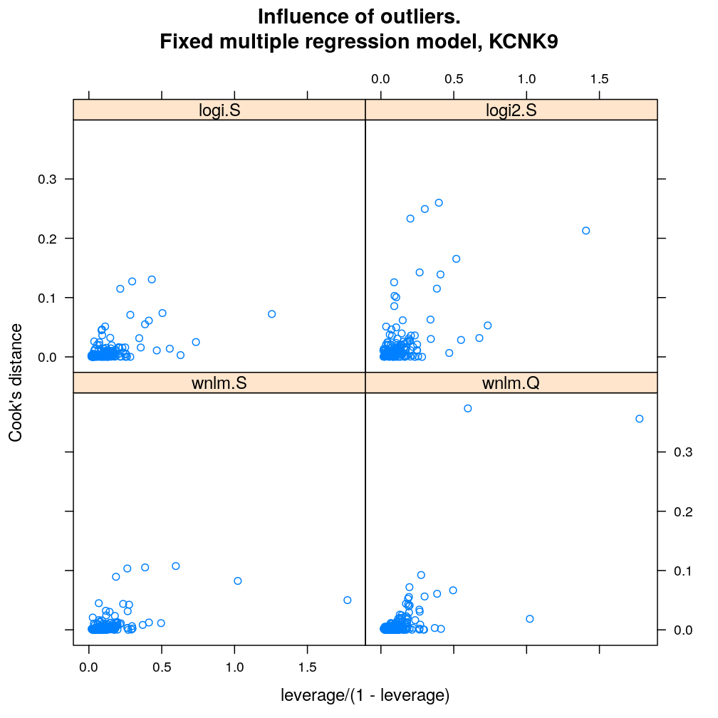
Here Cook’s distance is plotted against , where the leverage of case (individual) is the -th element of the diagonal of the (weighted) projection matrix . The definition is
where is the number of parameters (see Statistical Models, p477).
So Cook’s distance combines the influence of case based on both the response (i.e. the residual ) and the predictors (more precisely the leverage , which for lm only depends on the predictors and for glm depends also on the response to some degree). Good fit is indicated by equally low (and ) for all cases implying that all cases carry equal amount of information on the regression parameters .
myinfluence <- function(mtype, xlim = c(-0.2, 4), ylim = c(-0.04, 0.8), skip = FALSE, ...)
    xyplot(cooks.dist ~ leverage / (1 - leverage) | gene, data = diagnostics, xlim = xlim, ylim = ylim,
           par.settings = list(add.text = list(cex = 0.8)),
           skip = skip, layout = c(6, 5),
           subset = model.type %in% mtype, pch = "+", main = mtype, ylab = "Cook's distance", ...)[c(1:30)[! skip]]

#myinfluence("unlm.S")
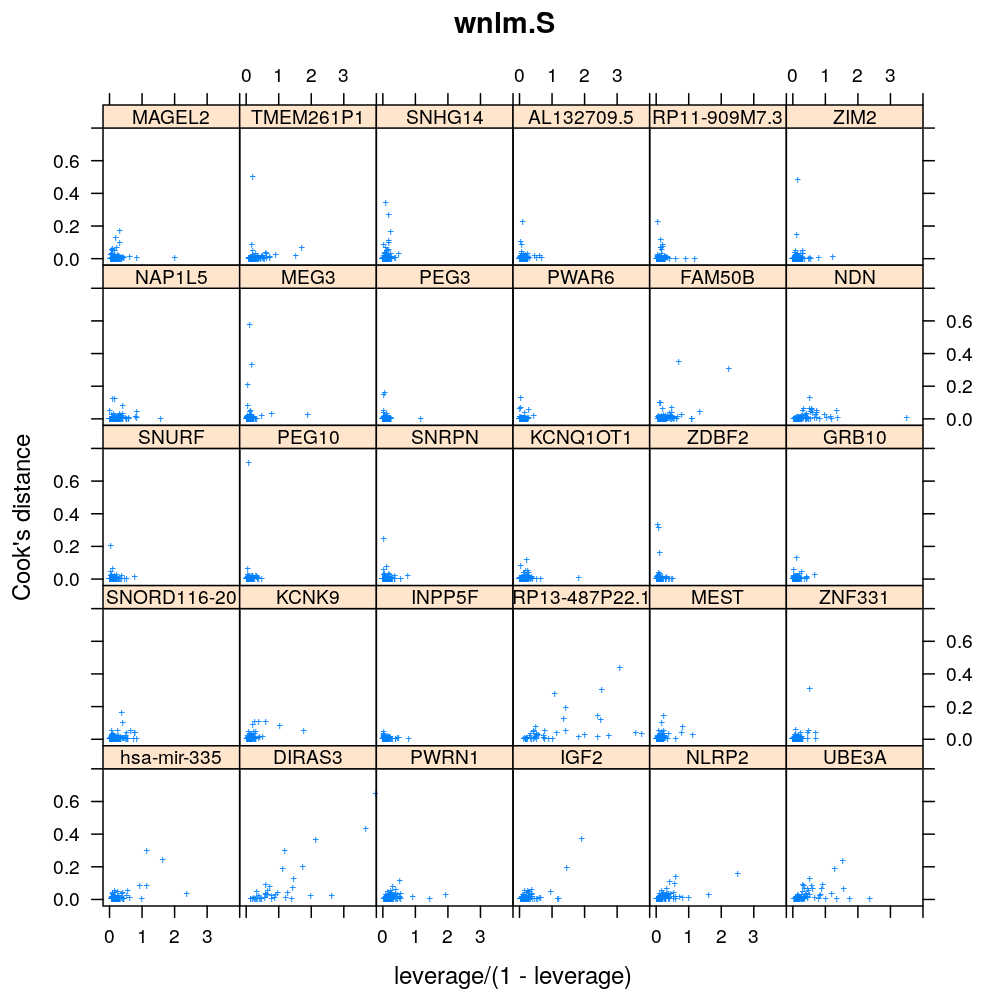
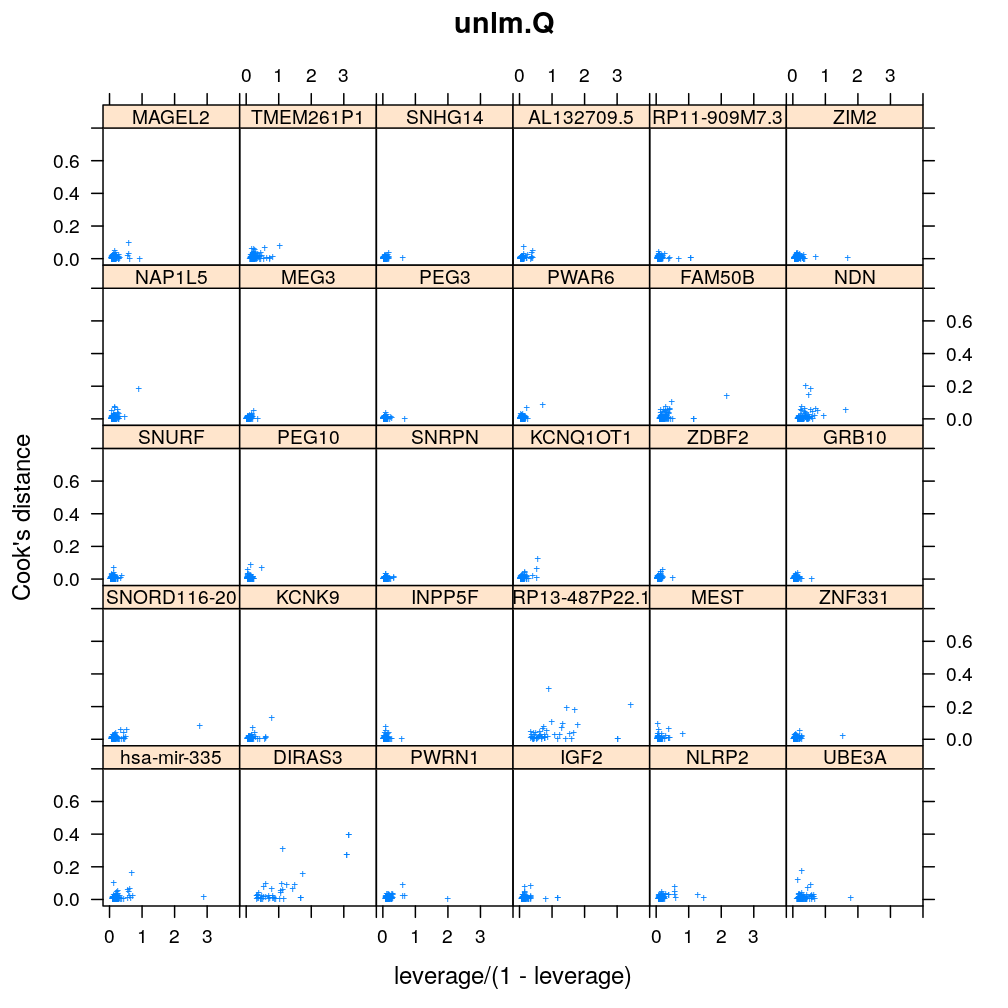
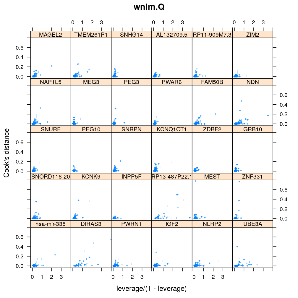
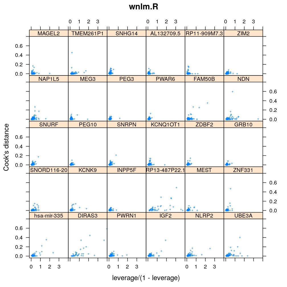
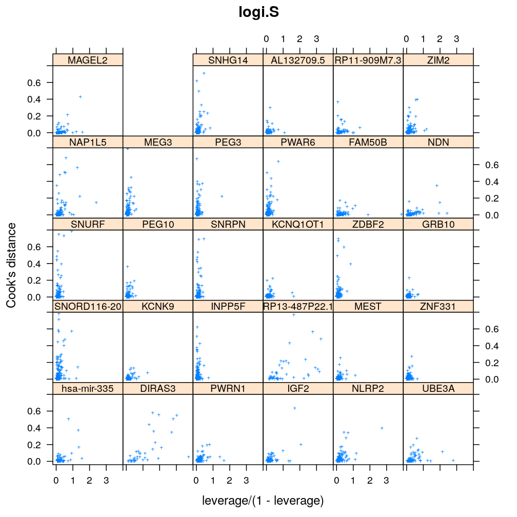
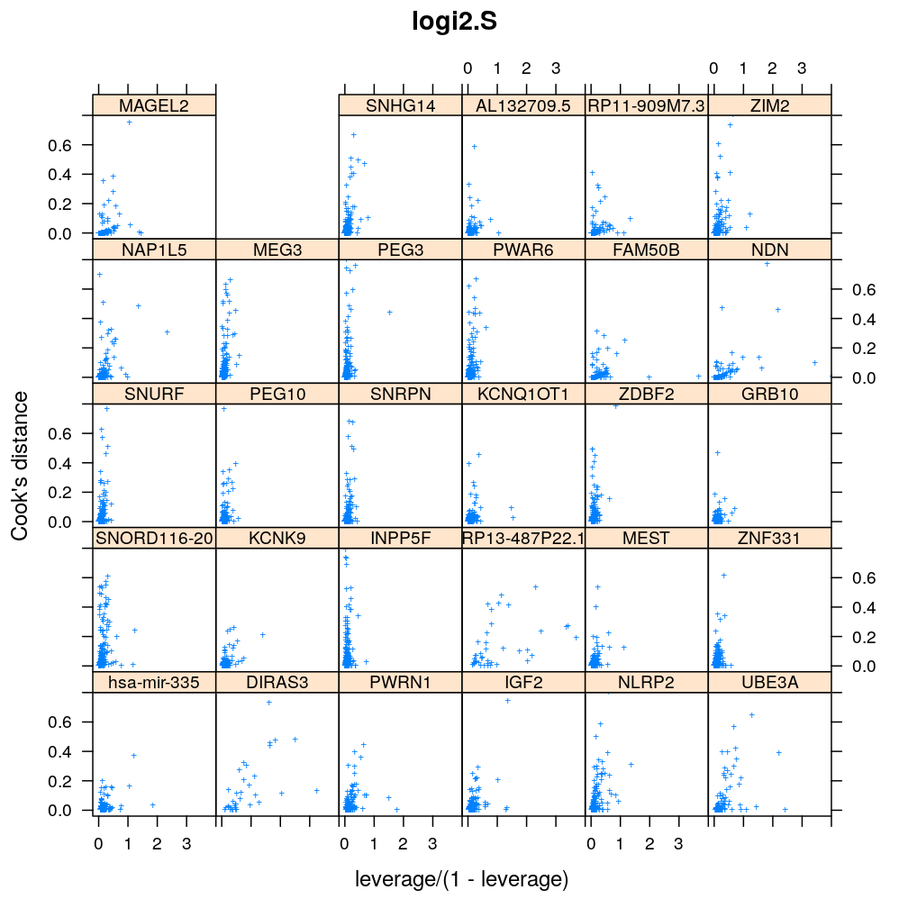
Figure for presentation
myinfluence.demo <- function(g) {
    xyplot(cooks.dist ~ leverage / (1 - leverage) | model.type, data = diagnostics,
           subset = gene == g & model.type != "wnlm.R", ylab = "Cook's distance",
           main = paste("Influence of outliers.
Fixed multiple regression model,", g))[c(1:2, 5, 4)]
}
myinfluence.demo("ZNF331")
myinfluence.demo("PEG3")
myinfluence.demo("ZDBF2")
myinfluence.demo("KCNK9")
Identifying outliers
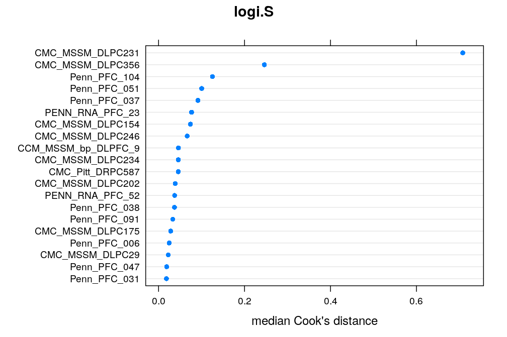
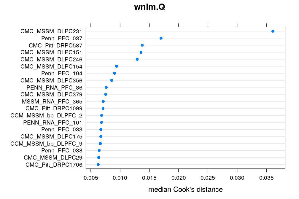
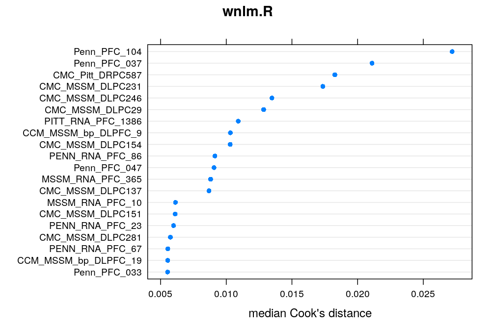
Here the median Cook’s distance taken across all 30 genes (with possibly missing values) for any given case/individual is used to quantify the overall impact of that case. The top 20 cases are shown under each model. CMC_MSSM_DLPC231 tops the list both under logi.S and wnlm.Q but there are several other cases which rank within the top 20 under both models. Exclusion of some of these might substantially improve model fit for some genes.
cooks.d <- lapply(M, function(m)
                  as.matrix(data.frame(lapply(m[gene.ids], get.influence, rownames(E)))))
med.cooks.d <- lapply(cooks.d,
                      function(d) sort(apply(d, 1, median, na.rm = TRUE), decreasing = TRUE))
dotplot(rev(med.cooks.d$logi.S[1:20]), main = "logi.S", xlab = "median Cook's distance")
Decision on model fit
Considering the two preferred models, wnlm.Q and logi.S, the following decision has been made in light of the results above:
- wnlm.Q fit is accepted for all genes
- logi.S fit is accepted for only some genes, printed below:
read.csv("../../results/model-checking.csv", row.names = "gene")[-4]
##               residuals.normal homoscedasticity influence logi.S.fit.OK
## MAGEL2                     0.0              0.0         1         FALSE
## TMEM261P1                  0.0              0.0         0         FALSE
## SNHG14                     0.0              0.5         0         FALSE
## AL132709.5                 0.5              0.5         1         FALSE
## RP11-909M7.3               0.0              0.0         1         FALSE
## ZIM2                       0.0              0.5         1         FALSE
## NAP1L5                     0.5              1.0         0         FALSE
## MEG3                       0.0              0.5         0         FALSE
## PEG3                       0.0              1.0         0         FALSE
## PWAR6                      0.0              0.5         0         FALSE
## FAM50B                     0.5              0.5         1         FALSE
## NDN                        0.5              0.5         1         FALSE
## SNURF                      0.0              0.5         0         FALSE
## PEG10                      0.0              0.5         1         FALSE
## SNRPN                      0.0              0.5         0         FALSE
## KCNQ1OT1                   1.0              1.0         1          TRUE
## ZDBF2                      0.0              0.5         0         FALSE
## GRB10                      1.0              1.0         1          TRUE
## SNORD116-20                0.0              1.0         0         FALSE
## KCNK9                      1.0              1.0         1          TRUE
## INPP5F                     0.0              0.5         0         FALSE
## RP13-487P22.1              1.0              1.0         0         FALSE
## MEST                       1.0              1.0         1          TRUE
## ZNF331                     0.5              1.0         1         FALSE
## hsa-mir-335                1.0              1.0         1          TRUE
## DIRAS3                     1.0              1.0         0         FALSE
## PWRN1                      1.0              1.0         1          TRUE
## IGF2                       1.0              1.0         1          TRUE
## NLRP2                      0.5              1.0         1         FALSE
## UBE3A                      1.0              1.0         1          TRUE
As can be seen, all three criteria (normality of residuals, homoscedasticity, balanced influence of cases) had to be met for acceptable fit.