This analysis compares our findings on the biological regulation of parental expression bias to those published by Perez et al (eLife 2015;4:e07860), who presented and applied the BRAIM model to RNA-seq data from the cerebellum of P8 and P60 hybrid mice.
Preparation
Load functions
source("~/projects/monoallelic-brain/src/import-data.R")
source("~/projects/monoallelic-brain/src/fit-glms.R")
source("~/projects/monoallelic-brain/src/graphics.R")
Orthology: matching human and mouse genes
Import “associated names” (symbols) for the selected human genes:
h.g.names <- unlist(read.csv("../../data/genes.regression.new", as.is = TRUE))
names(h.g.names) <- h.g.names
Import results by Perez et al provided in the first sheet of Supplementary file 1.
perez <- read.csv("../../data/elife-07860/elife-07860-supp1-v2.csv", as.is = TRUE)
Using AnnotationDbi
library(AnnotationDbi)
library("org.Hs.eg.db")
## Error in library("org.Hs.eg.db"): there is no package called 'org.Hs.eg.db'
library("org.Mm.eg.db")
## Error in library("org.Mm.eg.db"): there is no package called 'org.Mm.eg.db'
library("hom.Hs.inp.db")
An initial attempt with the AnnotationDbi::inpIDMapper function retrieved the id of only 3 mouse orthologs for the 30 selected genes. As a result of this frustrating result the following conversion hack was done. Mouse gene names were “humanified” by all-capitalization, i.e. using the rule: Mest (mouse) -> MEST (human). The detailed operations follow:
Convert for the 30 selected human genes the gene names (stored in h.g.names) into Ensemble gene ids. Then print the name of those genes for which the conversion failed.
human.eg.ids <- unlist(as.list(org.Hs.egSYMBOL2EG[mappedkeys(org.Hs.egSYMBOL2EG)])[h.g.names])
## Error in as.list(org.Hs.egSYMBOL2EG[mappedkeys(org.Hs.egSYMBOL2EG)]): object 'org.Hs.egSYMBOL2EG' not found
# the conversion failed for these genes:
names(h.g.names[! h.g.names %in% names(human.eg.ids)])
## Error in h.g.names %in% names(human.eg.ids): object 'human.eg.ids' not found
Import all mouse gene ids and symbols, do the conversion hack and check which human genes could not be converted:
# get all mouse genes
mouse.all <- as.list(org.Mm.egSYMBOL2EG[mappedkeys(org.Mm.egSYMBOL2EG)])
## Error in as.list(org.Mm.egSYMBOL2EG[mappedkeys(org.Mm.egSYMBOL2EG)]): object 'org.Mm.egSYMBOL2EG' not found
# "humanify" mouse gene names by all-capitalization, i.e. using the rule Mest (mouse) -> MEST (human)
names(mouse.all) <- toupper(names(mouse.all))
## Error in toupper(names(mouse.all)): object 'mouse.all' not found
# convert mouse gene names (i.e. symbols) to upper case and check for non-matching human gene symbols
names(h.g.names[! h.g.names %in% toupper(as.character(perez$gene_name))])
##  [1] "TMEM261P1"     "SNHG14"        "AL132709.5"    "RP11-909M7.3"
##  [5] "ZIM2"          "PWAR6"         "FAM50B"        "SNURF"
##  [9] "KCNQ1OT1"      "SNORD116-20"   "RP13-487P22.1" "ZNF331"
## [13] "hsa-mir-335"   "DIRAS3"        "PWRN1"         "NLRP2"
This result shows that 16 human genes could not be matched to any mouse ortholog. Below is a more principled and therefore more trusted approach using BioMart.
Using BioMart
This has been done with the web-based BioMart tool of Ensemble, which produced the following file
h2m <- read.csv("../../data/human-mouse-orthology.csv", as.is = TRUE)
str(h2m)
## 'data.frame':	37 obs. of  5 variables:
##  $ Ensembl.Gene.ID                           : chr  "ENSG00000162595" "ENSG00000145945" "ENSG00000106070" "ENSG00000167244" ...
##  $ Mouse.Ensembl.Gene.ID                     : chr  "" "ENSMUSG00000038246" "ENSMUSG00000020176" "ENSMUSG00000048583" ...
##  $ Mouse.orthology.confidence..0.low..1.high.: int  NA 1 1 1 1 1 NA 1 NA 1 ...
##  $ Mouse.associated.gene.name                : chr  "" "Fam50b" "Grb10" "Igf2" ...
##  $ Associated.Gene.Name                      : chr  "DIRAS3" "FAM50B" "GRB10" "IGF2" ...
# remove rows without mouse ortholog; also remove the column "Mouse.orthology.confidence..0.low..1.high."
h2m <- h2m[h2m$Mouse.Ensembl.Gene.ID != "", -3]
nrow(h2m) == length(unique(h2m$Mouse.associated.gene.name))
## [1] TRUE
rownames(h2m) <- h2m$Mouse.associated.gene.name
h2m[-1 * 1:2]
##         Mouse.associated.gene.name Associated.Gene.Name
## Fam50b                      Fam50b               FAM50B
## Grb10                        Grb10                GRB10
## Igf2                          Igf2                 IGF2
## Inpp5f                      Inpp5f               INPP5F
## Kcnk9                        Kcnk9                KCNK9
## Magel2                      Magel2               MAGEL2
## Mest                          Mest                 MEST
## Nap1l5                      Nap1l5               NAP1L5
## Ndn                            Ndn                  NDN
## Nlrp2                        Nlrp2                NLRP2
## Peg10                        Peg10                PEG10
## Peg3                          Peg3                 PEG3
## Snrpn                        Snrpn                SNRPN
## Gm38393                    Gm38393                SNURF
## Snurf                        Snurf                SNURF
## Ube3a                        Ube3a                UBE3A
## Zdbf2                        Zdbf2                ZDBF2
Results
The results of Perez et al
Bringing the data table into a long format for plotting:
vname.pp <- paste0("posterior_mean.pp_", fc <- c("parent", "sex", "cross", "age"), "_effect")
vname.beta <- paste0("posterior_mean.", fc,  "_effect")
perez.l <- # long format
    reshape(perez[c("gene_name", vname.pp, vname.beta)], # extract variables of interest
            v.names = c("P", "beta"),
            direction = "long", varying = list(vname.pp, vname.beta), timevar = "predictor", times = fc, idvar = "id1")
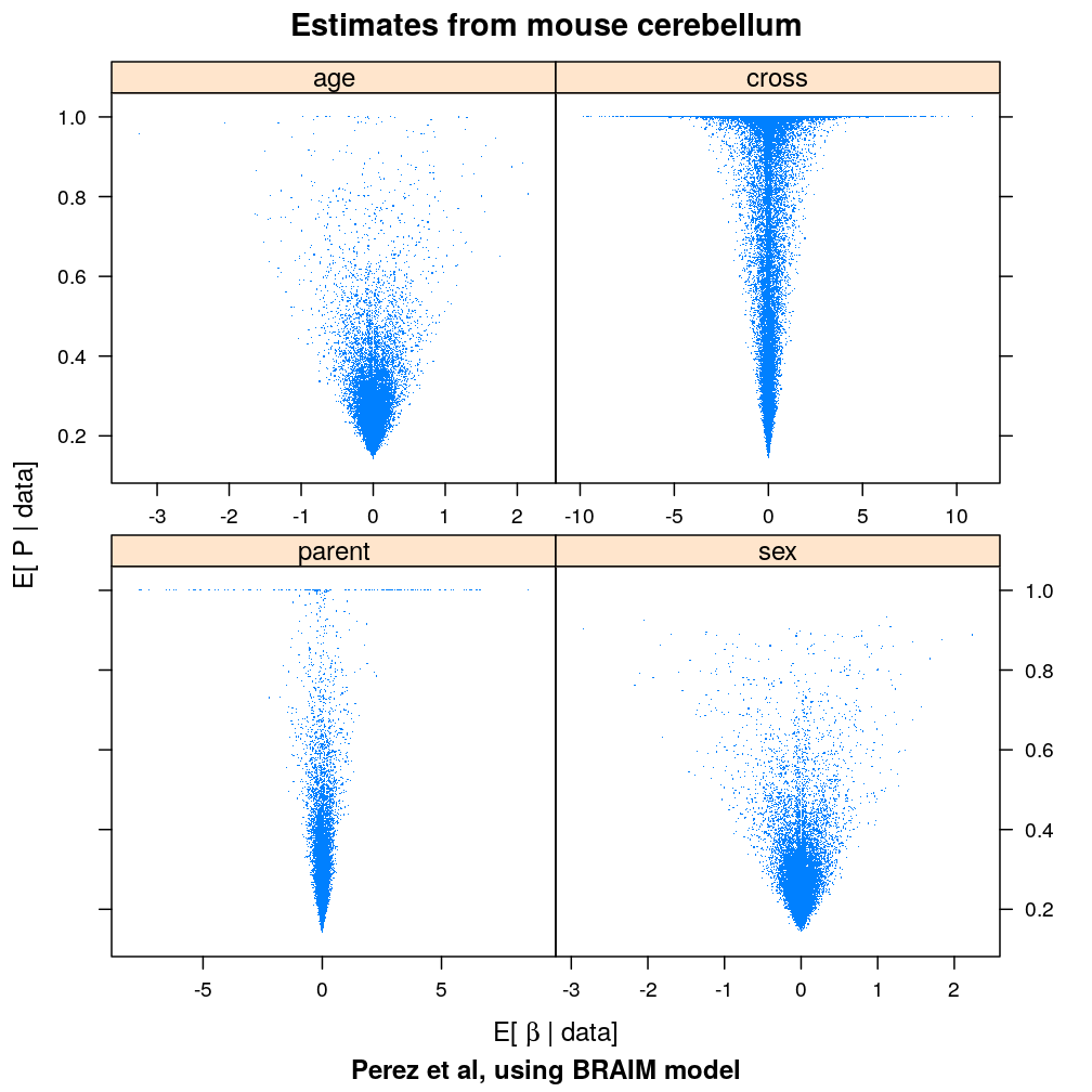
Plotted are posterior means of two parameters of the BRAIM model:
- , the regression coefficient mediating the effect of predictor for the parental bias of gene ; this is called
posterior_mean.age_effect,posterior_mean.sex_effect,…, in the first sheet of Supplementary file 1 provided by Perez et al. - , the probability that explanatory variable has large effect on parental bias of (i.e. induces a larger variance of ); this is called
posterior_mean.pp_age_effect,posterior_mean.pp_sex_effect,…,
xyplot(P ~ beta | predictor, data = perez.l, scales = list(x = list(relation = "free")), pch = ".",
       xlab = expression(paste("E[ ", beta, " | data]")), ylab = "E[ P | data]",
       sub = "Perez et al, using BRAIM model",
       main = "Estimates from mouse cerebellum")

This plot shows that the posterior mean of a regression coefficient need not differ greatly from zero even if provides a strong evidence that predictor significantly influences gene . This follows from the property of the BRAIM model that controls only the variance of but not its mean.
Comparison between the two studies
The following expressions focus only two predictors of parental bias: age and gender because only these two are clearly shared by our human study and the mouse study by Perez et al.
Data manuiplations
perez.s <- perez[perez$gene_name %in% h2m$Mouse.associated.gene.name, # rows: orthologs of selected human genes
                 c("gene_name", # informative columns
                   "posterior_mean.age_effect", "posterior_mean.pp_age_effect",
                   "posterior_mean.sex_effect", "posterior_mean.pp_sex_effect")]
perez.s <-
    do.call(rbind,
            lapply(unique(perez.s$gene_name),
                   function(n) {
                       df <- perez.s[ perez.s$gene_name == n, ]
                       cbind(data.frame(mouse.gene_name = n),
                             data.frame(t(as.matrix(apply(df[ , -1], 2, mean, na.rm = TRUE)))))
                   }))
perez.s$mouse.gene_name <- as.character(perez.s$mouse.gene_name)
rownames(perez.s) <- h2m[perez.s$mouse.gene_name, "Associated.Gene.Name"]
Combine evidence for the effect of age and gender from both our human study and the mouse study by Perez et al. The two types of evidence are:
- p-value for rejecting under the wnlm.Q or logi.S model, calculated either from normal distribution theory or a random permutation test
- the posterior mean
# Age
combined.a <- cbind(extractor("wnlm.Q", coef = "Age"),
                  extractor("logi.S")[-1 * c(1:2)])
combined.a <- cbind(combined.a,
                  expander("posterior_mean.age_effect", "beta.post.mean", df.long = combined.a),
                  expander("posterior_mean.pp_age_effect", "pp.post.mean", df.long = combined.a))
# Gender
combined.g <- cbind(extractor("wnlm.Q", coef = "GenderMale"),
                  extractor("logi.S")[-1 * c(1:2)])
combined.g <- cbind(combined.g,
                  expander("posterior_mean.sex_effect", "beta.post.mean", df.long = combined.g),
                  expander("posterior_mean.pp_sex_effect", "pp.post.mean", df.long = combined.g))
combined <- rbind(combined.a, combined.g)
The main result
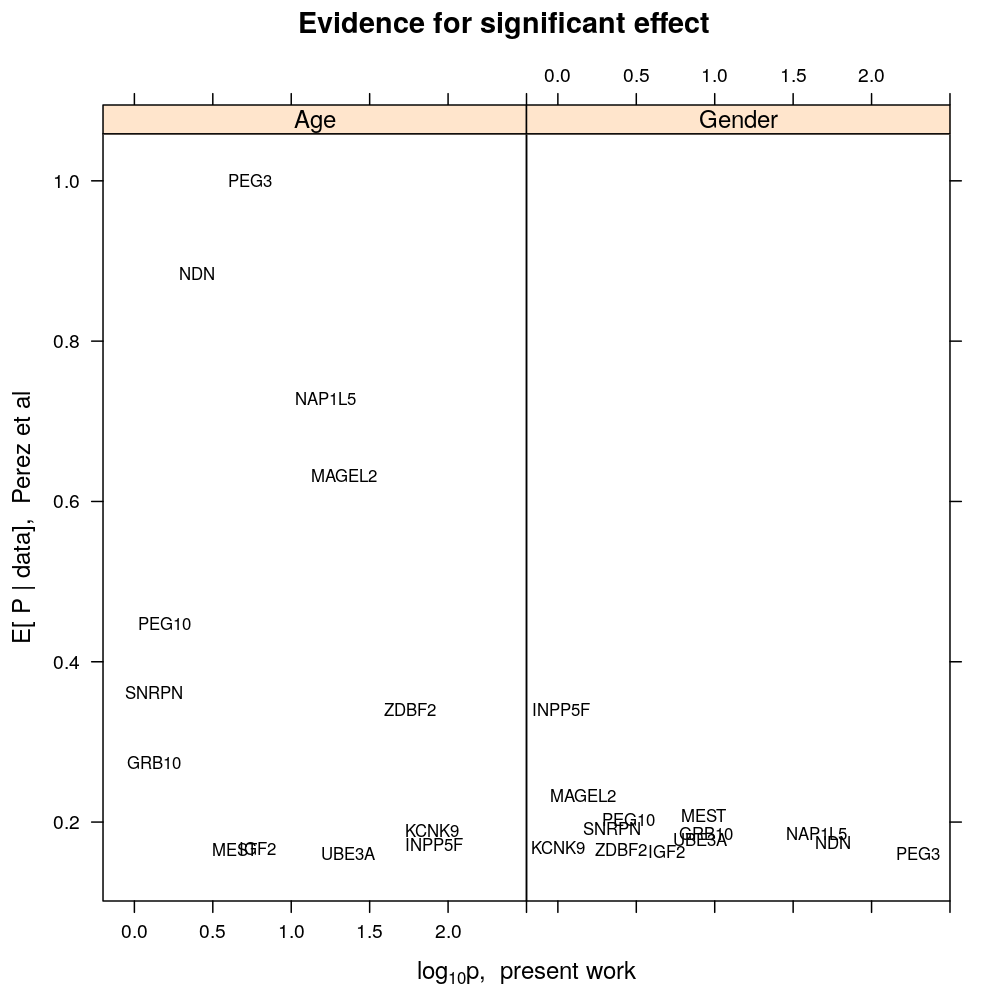
Plotted below is from Perez et al against , the p-value, from our study.
xyplot(pp.post.mean ~ - log10(p.val.t.dist.wnlm.Q) | Coefficient, data = combined, groups = Gene,
       panel = function(x, y, ..., groups) {
           panel.text(x, y, labels = groups, cex = 0.7, ...)
       },
       strip = strip.custom(factor.levels = c("Age", "Gender")),
       xlim = c(-0.2, 2.5),
       #aspect = 1,
       main = "Evidence for significant effect",
       xlab = expression(paste(log[10], p, ",  present work")),
       ylab = "E[ P | data],  Perez et al"
       )

Clearly, the evidence from the mouse and human study for any gene do not match each other. While there is evidence for some genes from both studies that age has an effect, only our human study detected significant effect of gender. These results suggests large differences between the studies, which are methodological and/or biological in nature. In particular:
- the RNA-seq data is modeled differently so the interpretation of the (BRAIM) is not identical to (wnlm.Q)
- differences in species, age window (relatively young mice vs relatively older people), and brain region
- differing measurement protocols