For certain genes allelic bias was found to depend on biological predictors (Age, Dx, Ancestry) in our previous analysis. That analysis fitted various fixed effects multiple regression models (GLM family) using as response variable the read count ratio or its quasi-log transformed version . After checking model fit, we primarily based our results to a weighted, normal linear model using , which we called wnlm.Q (as opposed to its unweighted variation unlm.Q). Significant dependence of the allelic bias of gene on (some level of) the predictor was assessed in terms of the estimated regression coefficient .
But decomposition of variance using variancePartition showed that a predictor that significantly affected allelic bias for a certain gene did not necessarily explain substantial fraction of variance. This was the case in spite of using the same response and predictors in the mixed effects model for variancePartition as for fixed effects models like wnlm.Q. A notable difference is that the mixed effects model was based on the unweighted unlm.Q rather than the weighted wnlm.Q.
What is the reason for this discrepancy? This question can be approached based on two cases giving altogether four explanations:
- under the fixed effects model largely deviates from that under the mixed effects model because of
- treating certain predictors’ effect random instead of fixed impacts for other predictors
- weighting, which was used for the fixed effects model wnlm.Q but not for the mixed effects model
- programming bug
- under the fixed effects agrees with that under the mixed effects model
- in this case the discrepancy arises from the related but different quantities of the two analyses: significance of is established using a -statistic whereas variance partitioning operates with the fractional variance explained (more details below)
The analysis below excludes programming bug and appears to suggest that the discrepancy is due to a mixture of the remaining three explanations.
Calculations
library(variancePartition)
library(doParallel)
library(lattice)
library(latticeExtra)
lattice.options(default.args = list(as.table = TRUE))
lattice.options(default.theme = "standard.theme")
opts_chunk$set(dpi = 144)
opts_chunk$set(out.width = "700px")
opts_chunk$set(dev = c("png", "pdf"))
source("../../src/import-data.R")
source("../../src/graphics.R")
source("../../src/fit-glms.R")
Import data
# selected set of genes
gene.ids <- unlist(read.csv("../../data/genes.regression.new", as.is = TRUE))
names(gene.ids) <- gene.ids
# predictors
names(e.vars) <- e.vars
E <- get.predictors()[e.vars]
# response: Q, quasi-log transformed read count ratio
Y <- get.readcounts(gene.ids = gene.ids, count.thrs = 0)
Q <- data.frame(sapply(Y[gene.ids], getElement, "Q"), check.names = FALSE)
# response: S, untransformed
S <- data.frame(sapply(Y[gene.ids], getElement, "S"), check.names = FALSE)
# total read count, used as weights
N <- data.frame(sapply(Y[gene.ids], getElement, "N"), check.names = FALSE)
Fit various fixed effect models to data for 30 selected genes
M <- do.all.fits(Z = Y[gene.ids], G = E)
Define model formula for fitting using the fitVarPartModel
(fchar <- as.character(formula(M$unlm.Q$MEST)))
## [1] "~"
## [2] "Y"
## [3] "Age + Institution + Gender + PMI + Dx + RIN + RNA_batch + Ancestry.1 + Ancestry.2 + Ancestry.3 + Ancestry.4 + Ancestry.5"
fm <- list()
fm$fixed.1 <- as.formula(paste(fchar[1], fchar[3]))
fm$mixed.1 <- ~ Age + (1|Institution) + (1|Gender) + PMI + (1|Dx) + RIN +(1|RNA_batch) + Ancestry.1 + Ancestry.2 + Ancestry.3 + Ancestry.4 + Ancestry.5
fm$mixed.2 <- ~ Age + (1|Institution) + Gender + PMI + Dx + RIN +(1|RNA_batch) + Ancestry.1 + Ancestry.2 + Ancestry.3 + Ancestry.4 + Ancestry.5
Fit fixed and mixed effects models using variancePartition
M$fixed.1 <- fitVarPartModel(t(Q), fm$fixed.1, E)
M$mixed.1 <- fitVarPartModel(t(Q), fm$mixed.1, E)
## Projected memory usage: > 3.2 Mb
## Projected run time: ~ 0.05 min
# the next expressions give errors
M$mixed.1.w <- fitVarPartModel(t(Q), fm$mixed.1, E, weightsMatrix = t(N))
## Projected memory usage: > 3.2 Mb
## Projected run time: ~ 0.09 min
## Error in {: task 1 failed - "Invalid grouping factor specification, Institution"
M$mixed.2 <- fitVarPartModel(t(Q), fm$mixed.2, E)
## Projected memory usage: > 3 Mb
## Projected run time: ~ 0.02 min
## Error in checkModelStatus(fitInit, showWarnings = showWarnings, colinearityCutoff): Categorical variables modeled as fixed effect: Gender
## The results will not behave as expected and may be very wrong!!
Weights for fitting are expected from voom; using total read counts as weights failed with an error for some reason. Also, there’s an error, when some factors are treated to convey fixed while the others as random effects.
# extract variance partitions from model objects
vp <- lapply(M[c("fixed.1", "mixed.1")], function(m) extractVarPart(m))
# reshape into long format
vpl <- data.frame(lapply(vp, function(v) stack(v[ , c(e.vars, "Residuals")])$values))
vpl$predictor <- factor(rep(c(e.vars, "Residuals"), each = length(gene.ids)), ordered = TRUE, levels = c(e.vars, "Residuals"))
vpl$gene <- factor(rep(gene.ids, length(c(e.vars, "Residuals"))), ordered = TRUE, levels = gene.ids)
vpl <- cbind(vpl[c("predictor", "gene")], vpl[- grep("predictor|gene", names(vpl))])
vpll <- reshape(vpl, varying = c("fixed.1", "mixed.1"), v.names = "fractional.variance",
                timevar = "model.type", times = c("fixed.1", " mixed.1"), direction = "long")
Extract for each gene under each model:
coef.names <- names(coef(M$unlm.Q[[1]]))
cf <- data.frame(lapply(M[- length(M)],
                        function(l.m)
                            stack(lapply(l.m,
                                         function(m)
                                             coef(m)[ coef.names ]))$values))
cf$mixed.1 <-
    stack(lapply(M$mixed.1,
                 function(m)
                     unlist(coef(m)[[1]][1, , drop = TRUE])[ coef.names ]))$values
#cf$coefficient <- rep(coef.names, length(gene.ids))
cf$coefficient <- factor(rep(coef.names, length(gene.ids)), ordered = TRUE, levels = coef.names)
cf$gene <- factor(rep(gene.ids, each = length(coef.names)), ordered = TRUE, levels = gene.ids)
cf <- cbind(cf[c("coefficient", "gene")], cf[- grep("coefficient|gene", names(cf))])
Calculate 99% confidence intervals for each (also extracts ):
beta.hat.CI <- lapply(M[c("unlm.Q", "wnlm.Q")], get.estimate.CI)
Finally, load objects for plotting:
source("2017-02-14-beta-from-mixed-model.R")
Results
Recapitulation: regression coefficients
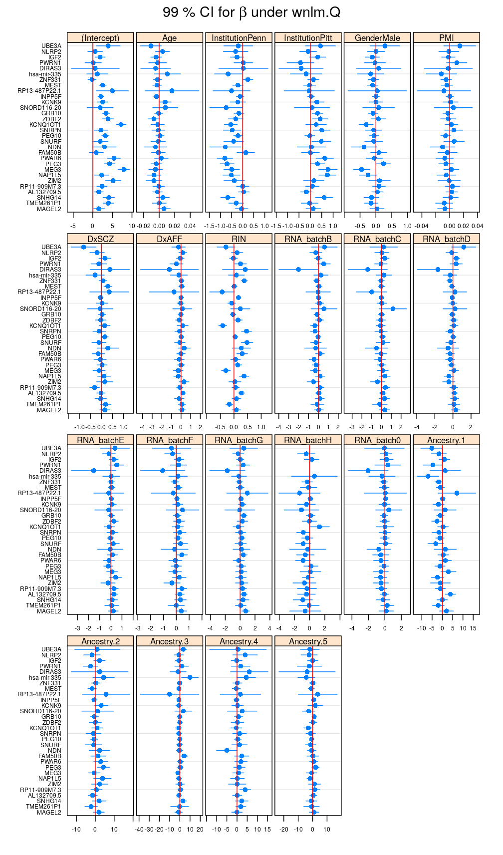
The plot below shows for each coefficient and gene the estimated regression coefficients and 99% confidence intervals (CI) for a under the wnlm.Q model. Note that these same results are presented in the current manuscript. Recall the close relationship between the CI and the p-value for rejecting the null hypothesis .

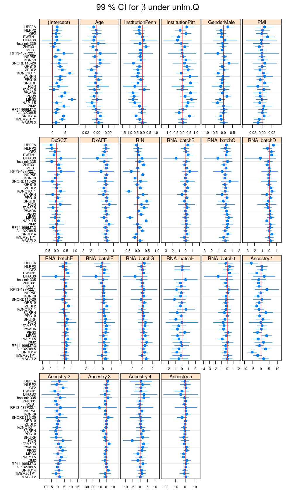
In the preceding calculations variance partitioning was based on not the wnlm.Q but the unlm.Q model, however. Therefore, a similar plot for the unlm.Q model comes next showing that weighting slightly changes and the CIs.
my.segplot(beta.hat.CI$unlm.Q, main = expression(paste("99 % CI for ", beta, " under unlm.Q")))

Variance partitioning
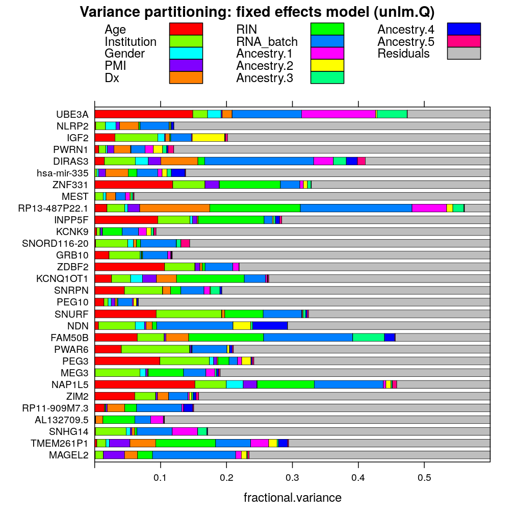
The next plot shows the fractional variance explained by each predictor for each gene under the fixed effects model unlm.Q.
tp <- trellis.par.get()
my.col <- c(rainbow(length(e.vars))[ c(seq(1, length(e.vars), by = 3), seq(2, length(e.vars), by = 3), seq(3, length(e.vars), by = 3)) ], "gray")
trellis.par.set(superpose.polygon = list(alpha = 1, col = my.col, border = "black", lty = 1, lwd = 0.5))
my.main <- "Variance partitioning: fixed effects model (unlm.Q)"
my.xlab <- "fractional variance"
barchart(gene ~ fractional.variance, data = vpll, groups = predictor, stack = TRUE, auto.key = list(columns = 3), xlim = c(0, 0.6), subset = model.type == "fixed.1", main = my.main)

Comparing coefficients to variance explained
Let be a predictor and a gene; the goal is to compare the set of regression the coefficient(s) to the fractional variance explained by . Note that the set of coefficients has only one member if predictor is a continuous variable or a factor with only one treatment level, in which case . In contrast, the set of coefficients has multiple members for factors with multiple treatment levels. Depending on the nature of predictor, the corresponding estimated coefficient(s) are on a particular scale. For this reason I use the t-statistic , which normalizes the coefficients across all predictors not only in the sense of placing them onto the same scale but also in the sense that the if then the corresponding p-values are also equal.
The plot indicates an expected positive correlation between and but the correlation is weakened by certain coefficients . Such coefficients are the 7 treatment levels (RNA_batchB,…, RNA_batch0) of the factor RNA_batch; each level has in itself relatively weak impact (small and hence weak significance) but together they explain relatively much variation. Another example for an outlier coefficient is that for Age, which again tends to have relatively small but large .
my.main <- "Quantities of effect size: fixed model (unlm.Q)"
my.xlab <- expression(paste(hat(sigma)[vg], " / ", hat(sigma)[tot], ", fractional variance explained"))
my.ylab <- expression(paste("|", t[pg], "|, normalized coefficient ", hat(beta)[pg]))
tval.vp.plot(tval.vp.data <- tval.vp(m.type = "fixed.1", llm = M), main = my.main, xlab = my.xlab, ylab = my.ylab)


For presentation
update(tval.vp.plot(tval.vp.data <- tval.vp(m.type = "fixed.1", llm = M), xlab = my.xlab, ylab = my.ylab)[c(5:8, 21:24)], layout = c(4, 2))

update(tval.vp.plot(tval.vp.data <- tval.vp(m.type = "fixed.1", llm = M), xlab = my.xlab, ylab = my.ylab)[c(3, 6, 14, 15, 24, 30)], layout = c(3, 2), key = my.key$coefficient.2)

Introducing random effects
The above results were obtained under unlm.Q, a fixed effects model. Turning all categorical (factor-type) predictors from fixed into random effects results in the mixed.1 mixed effects model. The next plot compares t-statistics to fractional variance under this model. Similar trend emerges as for the fixed effects model above but the positive correlation between and is stronger. This is partly due to removing multilevel factors, like RNA_batch, from the comparison (since their effects are modeled here as random) and partly to Age following more closely the trend displayed by other covariates. Subsequent plots will explore this in more detail.
my.main <- "Quantities of effect size: mixed model (mixed.1)"
tval.vp.plot(tval.vp.mixed.1 <- tval.vp(m.type = "mixed.1", llm = M), main = my.main, xlab = my.xlab, ylab = my.ylab)


Impact on variance partitioning
The next plot illustrates how introducing random effects changes variance partitioning in terms of fractional variance explained. Some predictors, like Age, PMI, Dx, or RNA_batch, explain less variation in the mixed effects model, while the residuals increase. This phenomenologically explains the stronger correlation between and seen above.
my.main <- "Variance partitioning: mixed vs fixed effects model"
my.xlab <- "fractional variance: fixed effects (unlm.Q)"
my.ylab <- "fractional variance: mixed effects (mixed.1)"
my.plot(x = "fixed.1", y = "mixed.1", group.by = "predictor", lbl.type = "gene", dt = vpl, main = my.main, xlab = my.xlab, ylab = my.ylab)

Another view on the same results: grouping by genes
update(my.plot(x = "fixed.1", y = "mixed.1", group.by = "gene", lbl.type = "predictor", dt = vpl, subset = vpl$predictor != "Residuals", main = my.main, xlab = my.xlab, ylab = my.ylab), scales = list(relation = "free"), layout = c(4, 4))


Impact on regression coefficients
The impact of introducing random effects on statistics (normalized ) is rather small:

The result is similar for unnormalized :


These differences really reflect the introduction of random effects and are not due to software bug because the two different implementations of the fitting of the same fixed effects model (unlm.Q) gives identical results:
with(cf, all.equal(unlm.Q, fixed.1))
## [1] TRUE
Introducing weighting
Because fitting weighted models using variancePartition failed (see Calculations above), the impact of weighting is only studied in terms of regression coefficients:

