Lab Notebook

The advantage of linear mixed models is demonstrated on a toy data (sleepstudy, bundled with R), in which study individuals act as grouping factors instead of genes. The mixed model is global in the sense that it may be fitted to the entire dataset covering all groups jointly. This is contrasted with local models fitted separately to each group, which is less powerful and tends to over fit the data. The mixed model is also contrasted with a fixed global model, in which the groups (individuals, genes) all have the same effect on the response or on the dependence of the response on predictors of potential interest.

library(lme4)

## Loading required package: Matrix

## Loading required package: methods

library(lattice)
lattice.options(default.args = list(as.table = TRUE))
lattice.options(default.theme = "standard.theme")
opts_chunk$set(dpi = 144)
opts_chunk$set(out.width = "700px")
opts_chunk$set(dev = c("png", "pdf"))

Demo

Data

The sleepstudy dataset from the lme4 package is chosen for the demonstration. Below is the description of sleepstudy

The average reaction time per day for subjects in a sleep deprivation study. On day 0 the subjects had their normal amount of sleep. Starting that night they were restricted to 3 hours of sleep per night. The observations represent the average reaction time on a series of tests given each day to each subject.

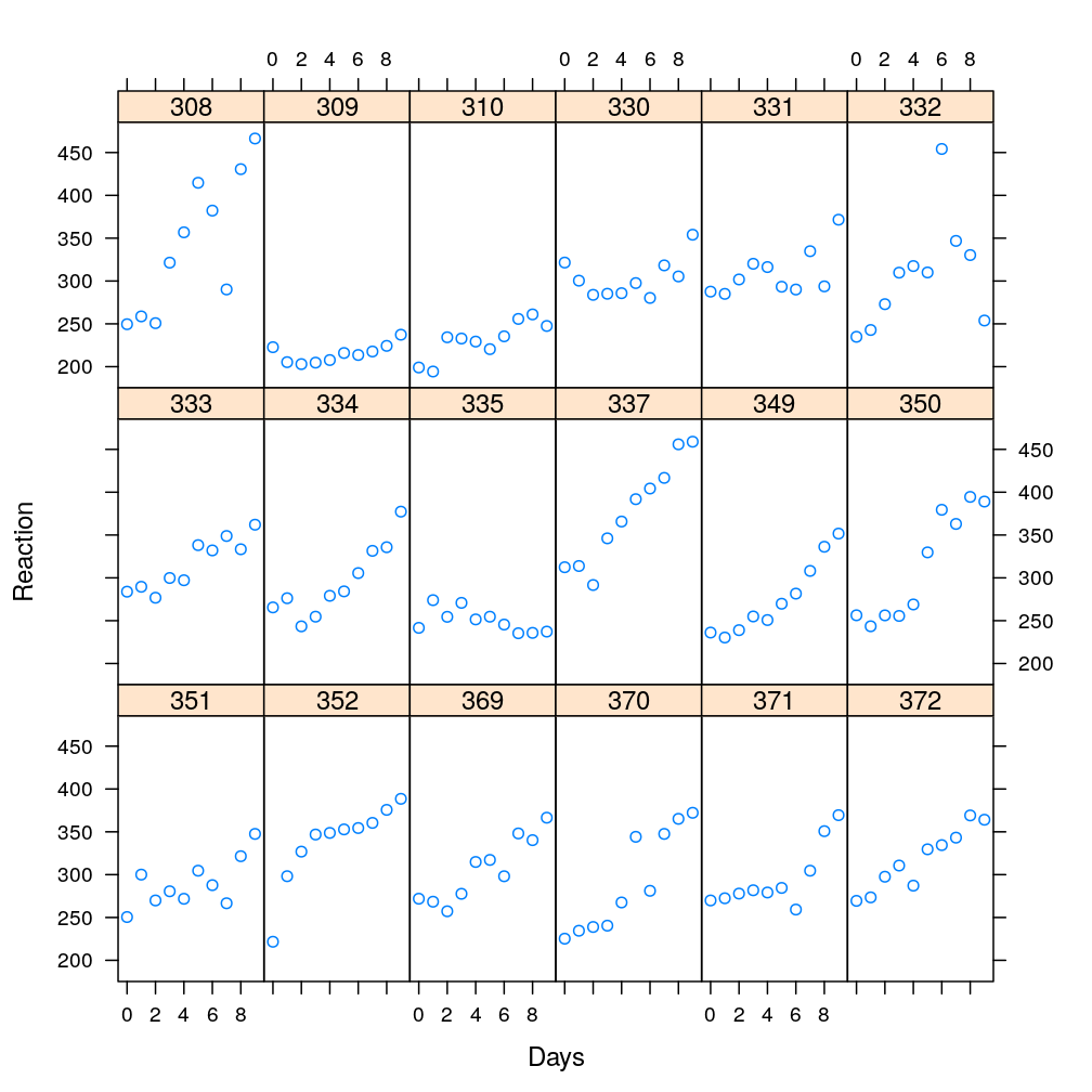
Plotting the average reaction time against the test day for each subject…

xyplot(Reaction ~ Days | Subject, data = sleepstudy, layout = c(6, 3))

We see that subjects appear to differ in terms of the average reaction time across all days; they also seem to differ in terms of how reaction time depends on the day. But subjects also share certain characteristics: for most subjects reaction time increases with days, and taken all days together, the average reaction time is somewhere around $300 ms$. We want to model both the shared characteristics as well as the heterogeneity among subjects.

Models

We consider two models, $M1$ and $M2$. These are nested: $M1 \supset M2$, meaning that $M1$ is more general while $M2$ is a constrained version of $M1$. Both models account for two shared characteristics among subjects: the increasing tendency of reaction time with days, captured by parameter $\beta$, as well as the roughly $300ms$ day- and subject-averaged reaction time, $\mu$. Moreover, both models also account for the subject-specific variation about $\mu$ by including a separate day-averaged reaction time parameter $\delta_g$ for each subject $g = 1,...,G$. However, only $M1$ allows for subject-specific dependence of reaction time on days, which is expressed by parameters $\gamma_1\neq...\neq\gamma_G$. In contrast, $M2$ assumes that subjects are identical in that respect so $\gamma_1=...=\gamma_G$.

After the above qualitative description we specify the models qualitatively. Both models share the following form and properties: $\begin{eqnarray*} y_{gi} &=& \mu + x_i (\beta + \gamma_g) + \delta_g + \varepsilon_{gi} \\\\ \delta \equiv (\delta_1, ..., \delta_G) &\sim& \mathcal{N}(0, \Omega_\delta) \\\\ \varepsilon_{gi} &\sim& \mathcal{N}(0, \sigma^2). \end{eqnarray*}$ In addition, $\beta$ is an unknown fixed parameter both in $M1$ and $M2$.

The only difference between $M1$ and $M2$ is $\gamma \equiv (\gamma_1, ..., \gamma_G)$; in $M1$ it is allowed to vary randomly while in $M2$ it is constrained to be 0: $\begin{eqnarray*} M1: \; \gamma &\sim& \mathcal{N}(0, \Omega_\gamma) \\\\ M2: \; \gamma &=& 0 \end{eqnarray*}$

M1 <- lmer(Reaction ~ Days + (Days | Subject), sleepstudy)
M2 <- lmer(Reaction ~ Days + (1 | Subject), sleepstudy)

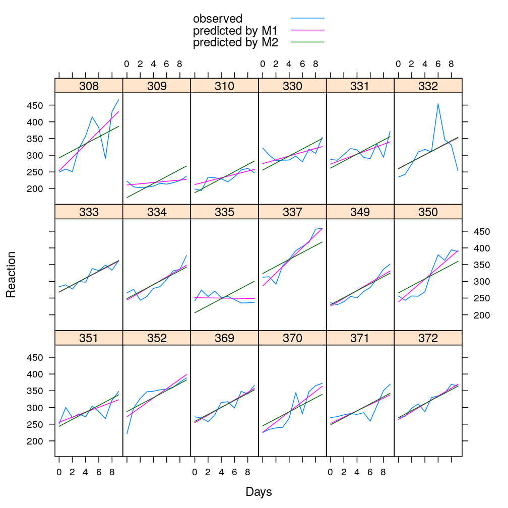
The magenta lines represent the fitted line under M1, the green lines under M2 (the observed data remain cyan).

df <- cbind(sleepstudy, data.frame(yhat.M1 = predict(M1), yhat.M2 = predict(M2)))
xyplot(Reaction + yhat.M1 + yhat.M2 ~ Days | Subject, data = df, type = "l", ylab = "Reaction", layout = c(6, 3),
       auto.key = list(text = c("observed", "predicted by M1", "predicted by M2"), points = FALSE, lines = TRUE))

Hypothesis testing

Does the dependence on days really vary across subjects or are subjects identical with respect to the dependence? We take the latter possibility as the null hypothesis $\begin{equation*} H_0 : \; \gamma_1\neq...\neq\gamma_G. \end{equation*}$

The most powerful test for $H_0$ is the likelihood ratio test comparing the M1 model to its constrained version M2:

anova(M1, M2)

## refitting model(s) with ML (instead of REML)

## Data: sleepstudy
## Models:
## M2: Reaction ~ Days + (1 | Subject)
## M1: Reaction ~ Days + (Days | Subject)
##    Df    AIC    BIC  logLik deviance  Chisq Chi Df Pr(>Chisq)    
## M2  4 1802.1 1814.8 -897.04   1794.1                             
## M1  6 1763.9 1783.1 -875.97   1751.9 42.139      2  7.072e-10 ***
## ---
## Signif. codes:  0 '***' 0.001 '**' 0.01 '*' 0.05 '.' 0.1 ' ' 1

Thus we may reject $H_0$ at significance level $<10^{-9}$ and conclude that the data supports overwhelmingly better the alternative hypothesis that the dependence of Reaction on Days varies across Subjects.

Implications to our study

Mixed models would afford joint modeling of the data across all 30 genes in a way that the effect of each predictor (e.g. Age) could possibly be divided into a global component (a fixed effect shared by all genes) and a gene-specific component (a gene-specific random effect). Compared to the previous strategy of separate gene-specific models the proposed joint modeling would extend the formally testable hypotheses to those that involve all genes jointly. Thus the main advantages would be

1. increased power of currently unresolved hypotheses e.g. the overall effect of Age taking all genes into account
2. more hypotheses may be tested by separating gene-specific effects from effects shared by all genes

Note that the increased power follows from the fact that joint modeling allows borrowing of strength from data across all genes and that powerful likelihood ratio tests could be easily formulated by comparing nested models. Additional benefits:

• better separation of technical and biological effects
  • for instance, we could model Institution-specific effect of RIN or RNA_batch and gene-specific effect of Age, Dx, or Ancestry.1
• shrinkage: for genes with many observations let the data “speak for themselves” but for data-poor genes shrink gene-specific parameters to a global average
• more straight-forward model comparison
  • various model families and data transformations
  • nested models (likelihood ratio tests)