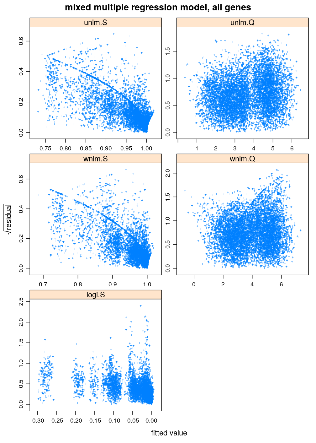
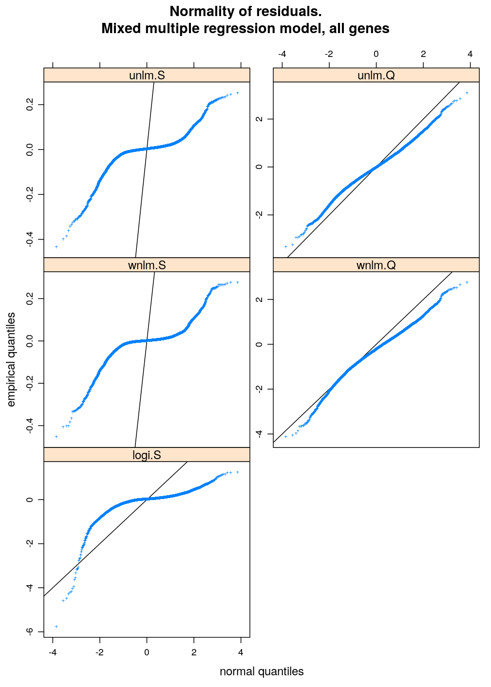
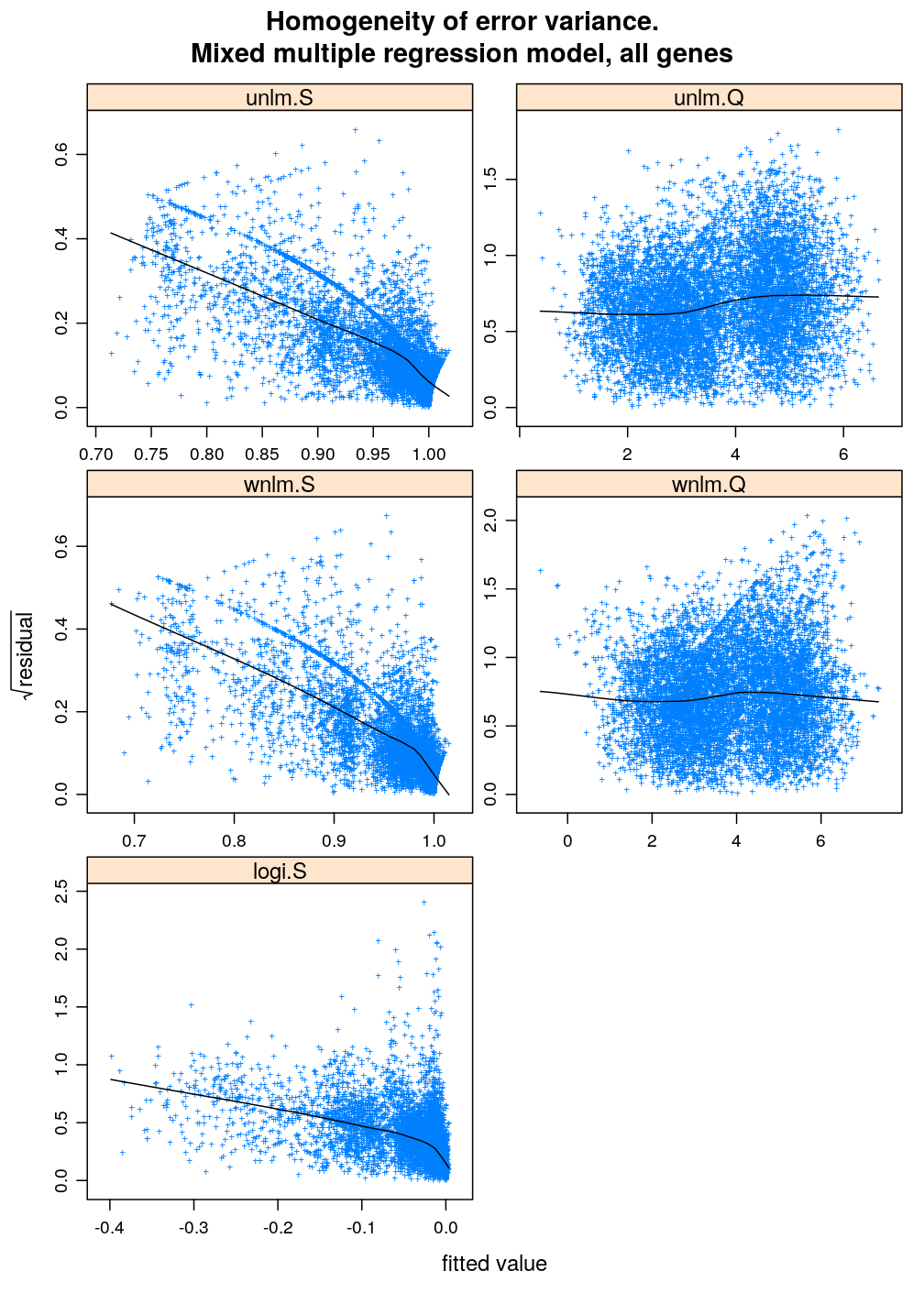
Two characteristics of fit are checked for a set of models: (1) normality of residuals and (2) homogeneity of error variance. These are evaluated with diagnostic plots. Among the checked models the best fitting one is unlm.Q and wnlm.Q regardless of the terms in the linear predictor. However, the fit of wnlm.Q converges very slowly or fails to converge especially when more terms are present in the linear predictor.
## Loading required package: Matrix
## Loading required package: methods
gene.ids <- unlist(read.csv("../../data/genes.regression.new", as.is = TRUE))
names(gene.ids) <- gene.ids
Prepare data frame including all 30 selected genes and read formulas (linear predictors) for models like the relatively simple and the more complex :
dat <- merge.data(gene.ids = gene.ids)
fm <- read.csv(file = "../../results/M-formulas.csv", stringsAsFactors = FALSE)
Results under
Fit models; note messages warning problems with convergence (slow convergence) for wnlm.Q and logi.S
M3 <- list()
M3$unlm.Q <- lmer(reformulate(fm$M3[3], response = "Q"), data = dat)
M3$wnlm.Q <- lmer(reformulate(fm$M3[3], response = "Q"), data = dat, weights = N)
## Warning in checkConv(attr(opt, "derivs"), opt$par, ctrl = control$checkConv, : Model is nearly unidentifiable: very large eigenvalue
##  - Rescale variables?
M3$unlm.S <- lmer(reformulate(fm$M3[3], response = "S"), data = dat)
M3$wnlm.S <- lmer(reformulate(fm$M3[3], response = "S"), data = dat, weights = N)
## Warning in optwrap(optimizer, devfun, getStart(start, rho$lower, rho$pp), :
## convergence code 1 from bobyqa: bobyqa -- maximum number of function
## evaluations exceeded
## Warning in checkConv(attr(opt, "derivs"), opt$par, ctrl = control
## $checkConv, : unable to evaluate scaled gradient
## Warning in checkConv(attr(opt, "derivs"), opt$par, ctrl = control
## $checkConv, : Model failed to converge: degenerate Hessian with 1 negative
## eigenvalues
M3$logi.S <- glmer(reformulate(fm$M3[3], response = "H.N"), data = dat, family = binomial)
## Warning in optwrap(optimizer, devfun, start, rho$lower, control =
## control, : convergence code 1 from bobyqa: bobyqa -- maximum number of
## function evaluations exceeded
## Warning in checkConv(attr(opt, "derivs"), opt$par, ctrl = control
## $checkConv, : unable to evaluate scaled gradient
## Warning in checkConv(attr(opt, "derivs"), opt$par, ctrl = control
## $checkConv, : Model failed to converge: degenerate Hessian with 1 negative
## eigenvalues
# do fit of simpler models to cache results right here
M1 <- list()
M1$unlm.Q <- lmer(reformulate(fm$M1[3], response = "Q"), data = dat)
M1$wnlm.Q <- lmer(reformulate(fm$M1[3], response = "Q"), data = dat, weights = N)
## Warning in checkConv(attr(opt, "derivs"), opt$par, ctrl = control$checkConv, : Model is nearly unidentifiable: very large eigenvalue
##  - Rescale variables?
M1$unlm.S <- lmer(reformulate(fm$M1[3], response = "S"), data = dat)
M1$wnlm.S <- lmer(reformulate(fm$M1[3], response = "S"), data = dat, weights = N)
## Warning in checkConv(attr(opt, "derivs"), opt$par, ctrl = control$checkConv, : Model is nearly unidentifiable: very large eigenvalue
##  - Rescale variables?
M1$logi.S <- glmer(reformulate(fm$M1[3], response = "H.N"), data = dat, family = binomial)
## Warning in checkConv(attr(opt, "derivs"), opt$par, ctrl = control
## $checkConv, : Model failed to converge with max|grad| = 0.00437736 (tol =
## 0.001, component 1)
## Warning in checkConv(attr(opt, "derivs"), opt$par, ctrl = control$checkConv, : Model is nearly unidentifiable: very large eigenvalue
##  - Rescale variables?
get.diagnostic.data <- function(lM, sel.col = 2:7) {
    helper <- function(x)
        cbind(data.frame(Residual = residuals(m <- lM[[x]]), Fitted.value = predict(m), Family = x),
              model.frame(m)[sel.col])
    l <- lapply(names(lM), helper)
    long <- do.call(rbind, l)
    lv <- c("unlm.S", "unlm.Q", "wnlm.S", "wnlm.Q", "logi.S")
    #lv <- c("logi.S", "unlm.S", "unlm.Q", "wnlm.S", "wnlm.Q")
    long$Family <- factor(long$Family, levels = lv, ordered = TRUE)
    return(long)
}
Normality of residuals
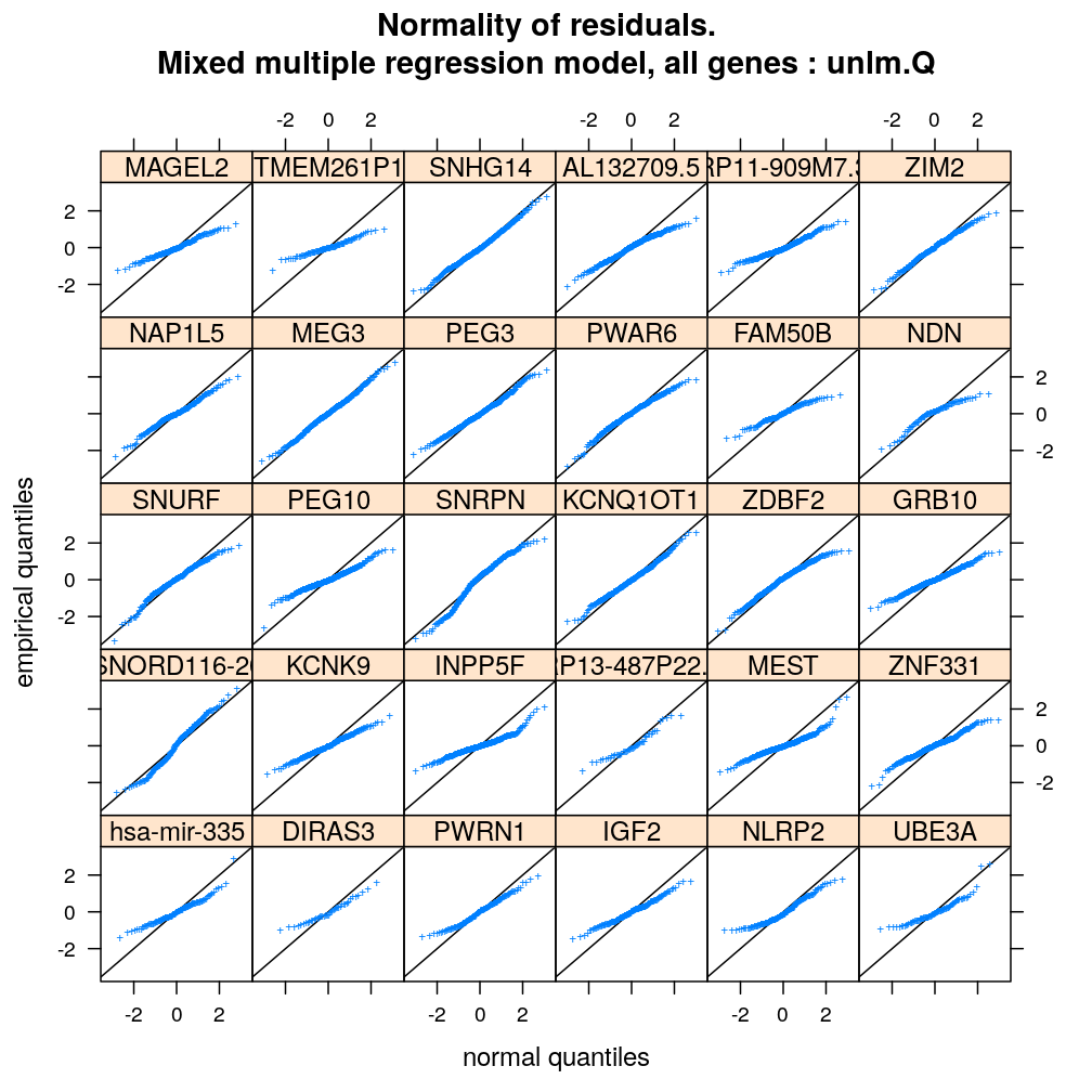
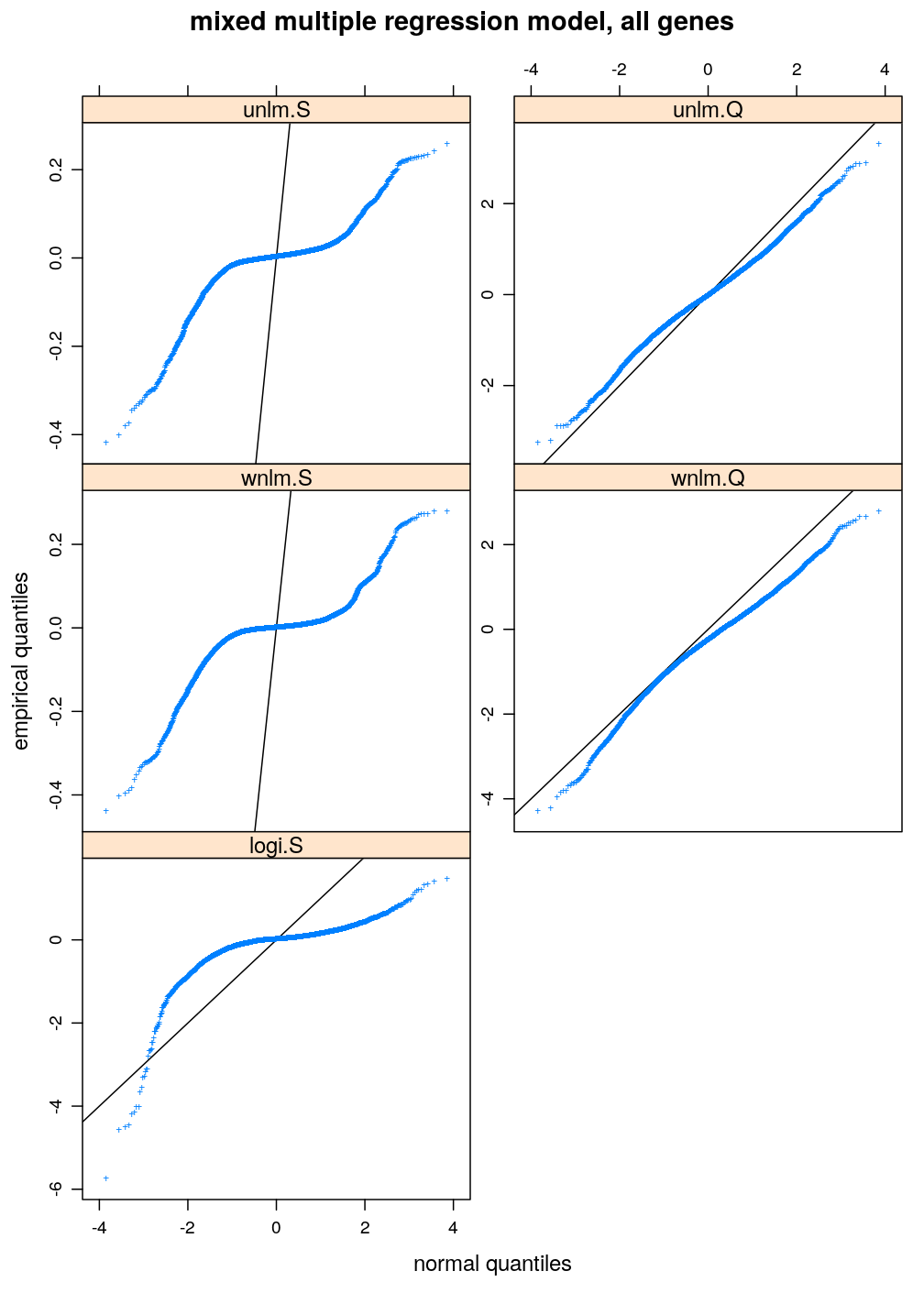
The distribution of residuals under all four model families shows smaller or larger departure from normality. unlm.Q is the closest to standard normal distribution and wnlm.Q is equally normal (or perhaps slightly less so). The distribution under logi.S is strikingly far from normal. So is it under unlm.S, for which additionally the scale of distribution is diminished (compare slope of black diagonal to the overall slope of the blue curve) indicating that the variance estimation—which is based on the residuals—is strongly biased downwards.
diag.M3 <- get.diagnostic.data(M3)
arg <- list(main = "Normality of residuals.
Mixed multiple regression model, all genes", xlab = "normal quantiles", ylab = "empirical quantiles", pch = "+")
qqmath(~ Residual | Family, data = diag.M3, scales = list(y = list(relation = "free")),
       xlab = arg$xlab, ylab = arg$ylab, main = arg$main, pch = arg$pch, abline = c(0, 1))
qqmath(~ Residual | Gene, data = diag.M3, subset = Family == "unlm.Q", xlab = arg$xlab, ylab = arg$ylab, main = paste(arg$main, ": unlm.Q"), pch = arg$pch, abline = c(0, 1))
Homogeneity of error
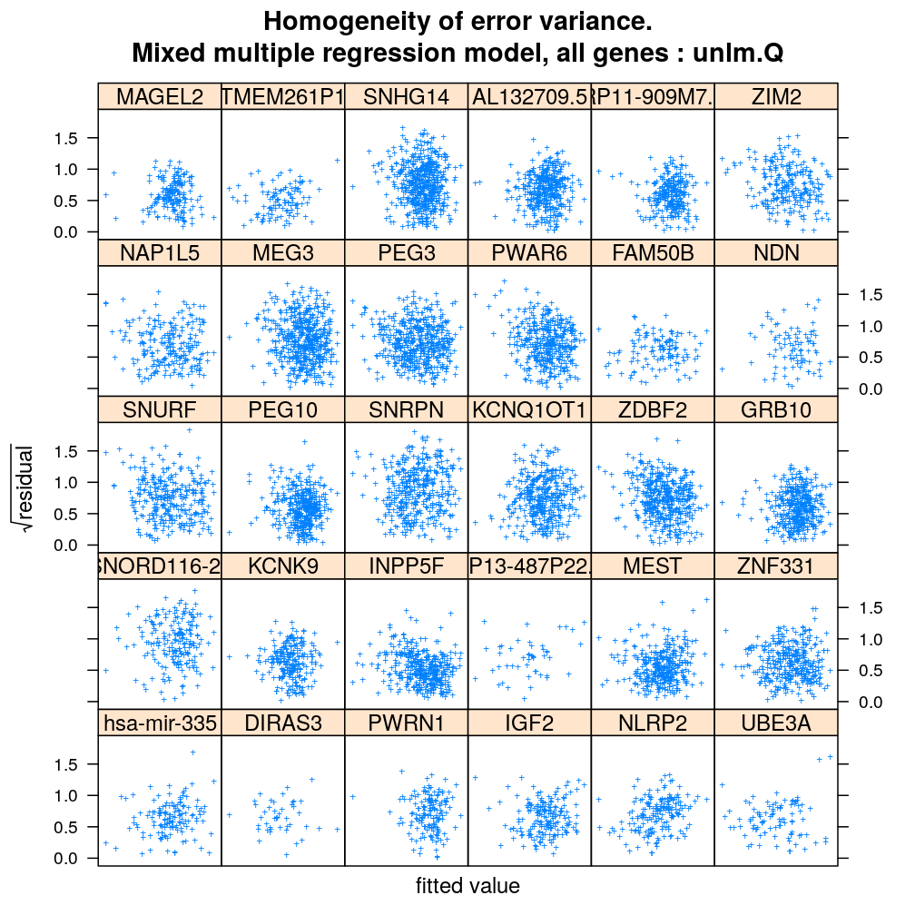
Inspecting the homogeneity of error variance (or equivalently standard deviation) leads to the same conclusion as above regarding the relative goodness of fit of the various model families: unlm.Q and wnlm.Q are the best (the most homoscedastic) while unlm.S and logi.S show systematic relationships between error and fitted value indicating poorer fit.
arg <- list(main = "Homogeneity of error variance.
Mixed multiple regression model, all genes", xlab = "fitted value", ylab = expression(sqrt(residual)), pch = "+")
xyplot(sqrt(abs(Residual)) ~ Fitted.value | Family, data = diag.M3, scales = list(relation = "free"),
       xlab = arg$xlab, ylab = arg$ylab, main = arg$main, pch = arg$pch,
       panel = function(...) { panel.xyplot(...); panel.loess(..., col = "black") })
xyplot(sqrt(abs(Residual)) ~ Fitted.value | Gene, data = diag.M3, subset = Family == "unlm.Q", scales = list(x = list(relation = "free", draw = FALSE)), xlab = arg$xlab, ylab = arg$ylab, main = paste(arg$main, ": unlm.Q"), pch = arg$pch)
Results under a simpler model,
Very similar patterns are seen under to those under . The fitting of the respective models from the wnlm.Q and logi.S families again converges with problems (see above).
diag.M1 <- get.diagnostic.data(M1)
arg <- list(main = "mixed multiple regression model, all genes", xlab = "normal quantiles", ylab = "empirical quantiles", pch = "+")
qqmath(~ Residual | Family, data = diag.M1, scales = list(y = list(relation = "free")),
       xlab = arg$xlab, ylab = arg$ylab, main = arg$main, pch = arg$pch, abline = c(0, 1))
arg <- list(main = "mixed multiple regression model, all genes", xlab = "fitted value", ylab = expression(sqrt(residual)), pch = "+")
xyplot(sqrt(abs(Residual)) ~ Fitted.value | Family, data = diag.M1, scales = list(relation = "free"),
       xlab = arg$xlab, ylab = arg$ylab, main = arg$main, pch = arg$pch)
