Lab Notebook

gene.ids <- unlist(read.csv("../../data/genes.regression.new", as.is = TRUE))
names(gene.ids) <- gene.ids
names(e.vars) <- e.vars
E <- get.predictors() # default arguments
Y <- get.readcounts(gene.ids = gene.ids, count.thrs = 0)

sel.models <- c("wnlm.Q", "unlm.Q", "logi.S")
M <- do.all.fits(Z = Y[gene.ids], G = E, preds = e.vars, sel.models = sel.models)

cf <- unlist(sapply(e.vars, function(e.v) predictor2coefs(M[[c(1, 1)]], e.v)))
p.val <-
    do.call(rbind,
            lapply(sel.models, function(mtype)
                   do.call(rbind,
                           lapply(cf, function(coef)
                                  do.call(rbind,
                                          lapply(gene.ids,
                                                 function(g) extract.p.val(mtype = mtype, gene = g, coef = coef, M = M)))))))

csv <- list(fixed = read.csv("../../results/regr-coefs.csv"),
            mixed = read.csv("../../results/anova-mixed-M5.csv"))

df <- list()
df$fixed <-
    subset(p.val, subset = Model %in% paste0(c("w", "u"), "nlm.Q") & Coefficient %in% c("DxSCZ", "Age", "Ancestry.1"),
           select = c(Model, Coefficient, Gene, p.val))
names(df$fixed) <- c("Model", "Predictor", "Term", "p")
df$mixed <-
    subset(csv$mixed, X %in% c("Dx", "Dx.Gene", "Age", "Age.Gene", "Ancestry.1", "Ancestry.1.Gene"),
           select = c(X, p.Chi))
df$mixed <- cbind(data.frame(Model = "M5", Predictor = sub(".Gene", "", df$mixed$X), df$mixed))
names(df$mixed) <- names(df$fixed)
df$mixed$Term <- c("{b_g}_g", "{b_g}_g", "{b_g}_g", "b", "beta", "beta")
df$mixed$Predictor <- sub("Dx", "DxSCZ", df$mixed$Predictor)
# Note fixed and mixed effects
df$fixed <- cbind(data.frame(Effects = "fixed"), df$fixed)
df$mixed <- cbind(data.frame(Effects = "mixed"), df$mixed)
# color
df$fixed$Color <- "red"
df$mixed <- cbind(df$mixed, data.frame(Color = rep(c("blue", "green4"), each = 3)))
# binding fixed and mixed results together
d <- droplevels(rbind(df$fixed, df$mixed))
d$Term <-
    factor(d$Term,
           levels = c(gene.ids, "beta", "b", "{b_g}_g"),
           ordered = TRUE)
d$Predictor <-
    factor(d$Predictor, levels = c("DxSCZ", "Age", "Ancestry.1"), ordered = TRUE)
pars <- list(fixed = gene.ids, mixed = setdiff(levels(d$Term), gene.ids))

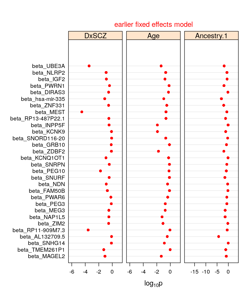
my.dotplot(do.mixed = FALSE, do.unlm.Q = FALSE)

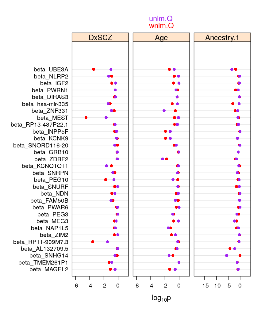
my.dotplot(do.mixed = FALSE, do.unlm.Q = TRUE)

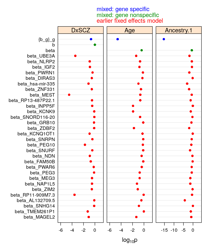
my.dotplot(do.mixed = TRUE, do.unlm.Q = FALSE)

beta.99.CI <-
    subset(read.csv("../../results/beta-99-CI.csv"),
           subset = Model == "wnlm.Q" & Coefficient %in% c("DxSCZ", "Age", "Ancestry.1"),
           select = c(Estimate, Lower.CL, Upper.CL, Gene, Coefficient))
beta.99.CI$Gene <- factor(beta.99.CI$Gene, levels = gene.ids, ordered = TRUE)
beta.99.CI$Coefficient <- factor(beta.99.CI$Coefficient, levels = levels(d$Predictor), ordered = TRUE)

my.segplot <- function(dt, param = pars, ...) {
    with(dt, dotplot(Gene ~ Estimate | Coefficient,
            prepanel = function(x, y, subscripts, ...)
                list(xlim = range(c(Lower.CL[subscripts], Upper.CL[subscripts]), na.rm = TRUE)),
            panel = function(x, y, groups, subscripts, ...) {
                panel.abline(v = 0, col = "cyan", lty = 1)
                lsegments(x0 = Lower.CL[subscripts], y0 = y, x1 = Upper.CL[subscripts], y1 = y, col = "red", ...)
                panel.xyplot(x, y, col = "red", pch = 16,...)
            },
            scales = list(x = list(relation = "free"),
                          y = list(limits = seq(from = 0, to = 4 + length(levels(dt$Gene))), at = seq_along(levels(dt$Gene)),
                                   labels = c(levels(dt$Gene), rep("", 3))
                                   )
                          ),
            auto.key = list(text = c("", "", "earlier fixed effects model"), col = "red", points = FALSE),
            between = list(x = 0.5),
            xlab = "beta_g: estimate and 99% conf. int.",
            layout = c(3, 1),
            ...))
}
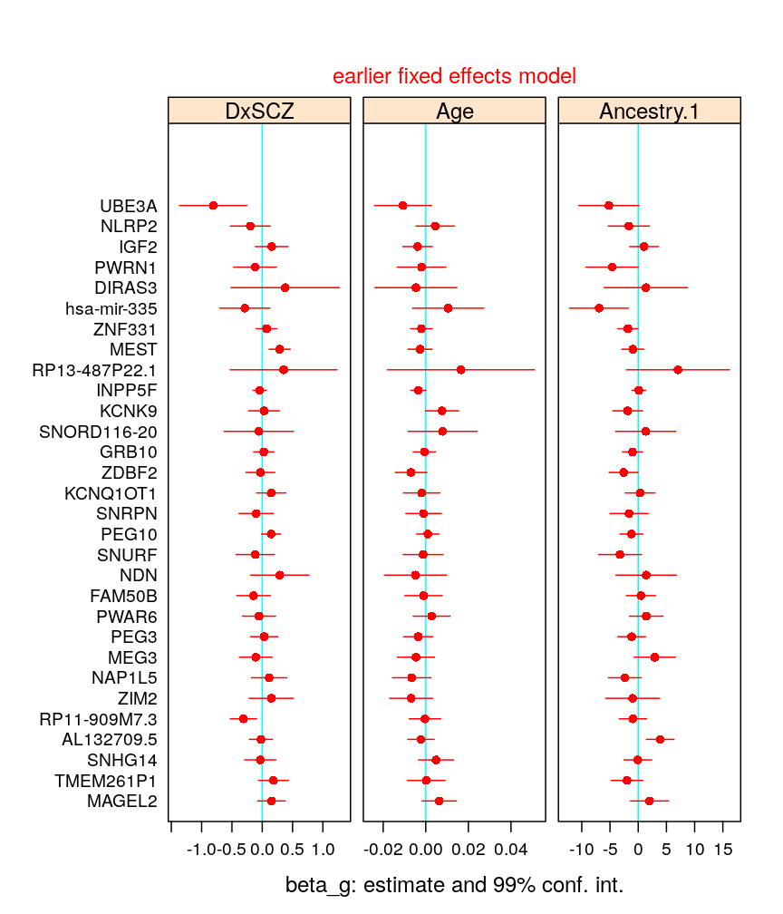
my.segplot(beta.99.CI)