This article illustrates some of the properties of the various regression models (logi.S, logi2.S, wnlm.S, wnlm.R, unlm.S, unlm.R) used to fit the Common Mind data as well as the properties of the data themselves
- link function: linear (wnlm.S, wnlm.R, unlm.S, unlm.R) and logit (logi.S, logi2.S)
- error distribution: normal (wnlm.S, wnlm.R, unlm.S, unlm.R) and binomial (logi.S, logi2.S)
- heteroscedasticity in data
See also 2016-04-22-glm-for-s-statistic.
Data preparation
## Loading required package: RColorBrewer
Load data importer functions:
source("../../src/import-data.R")
source("../../src/fit-glms.R")
source("2016-08-23-glm-sampling-distributions.R")
Do the import and fit all simple and multiple regression models as before (code hidden).
Results
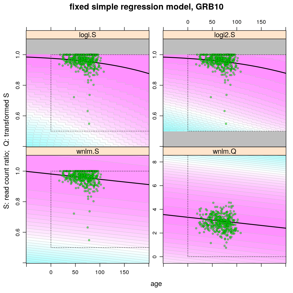
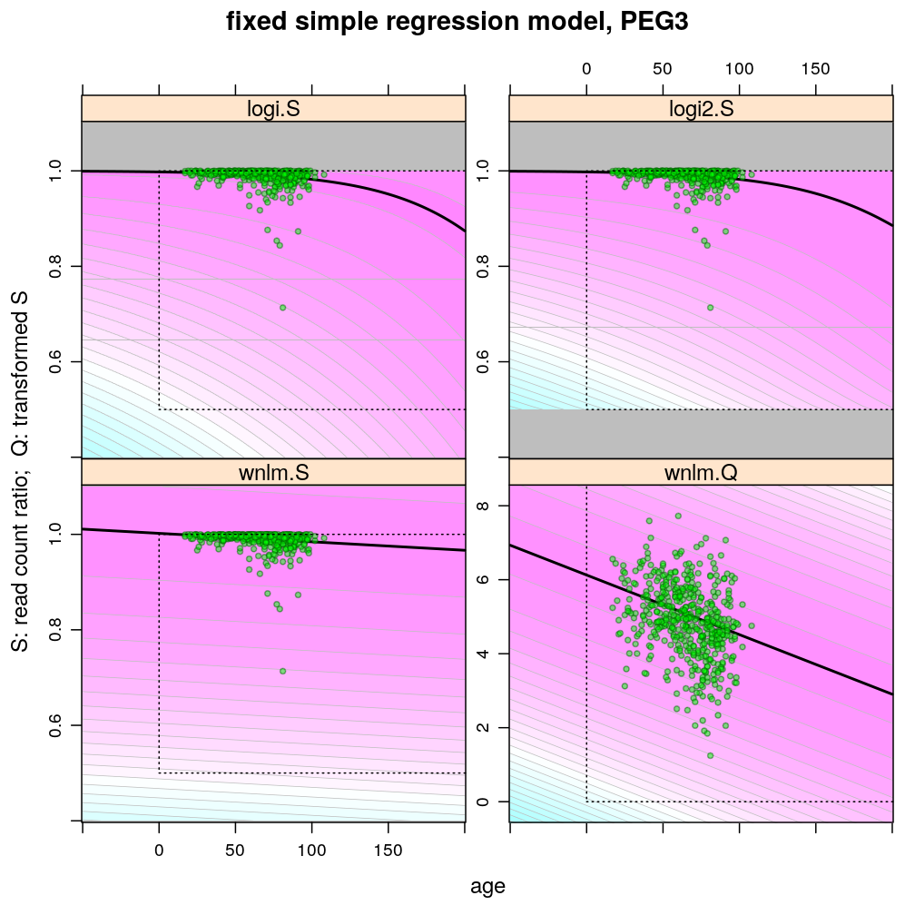
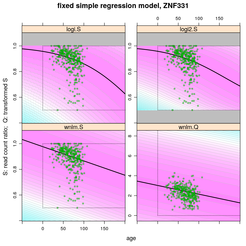
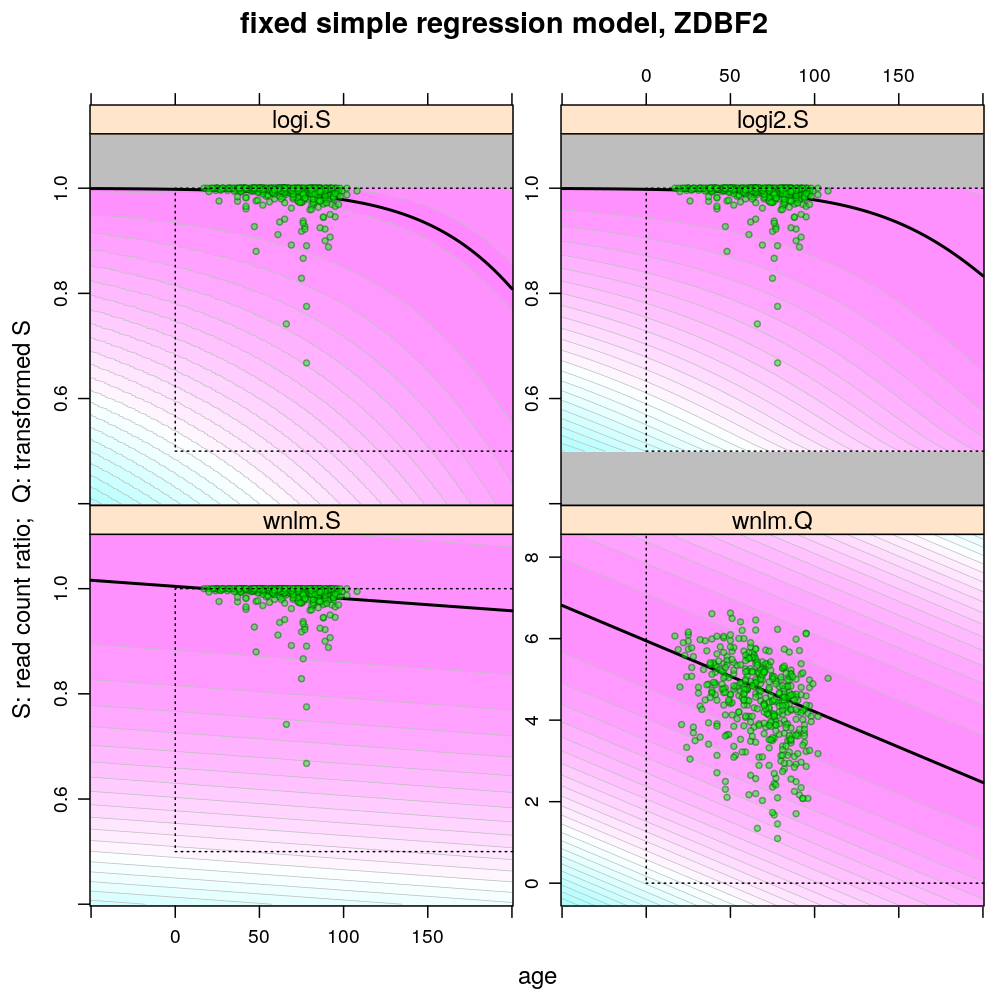
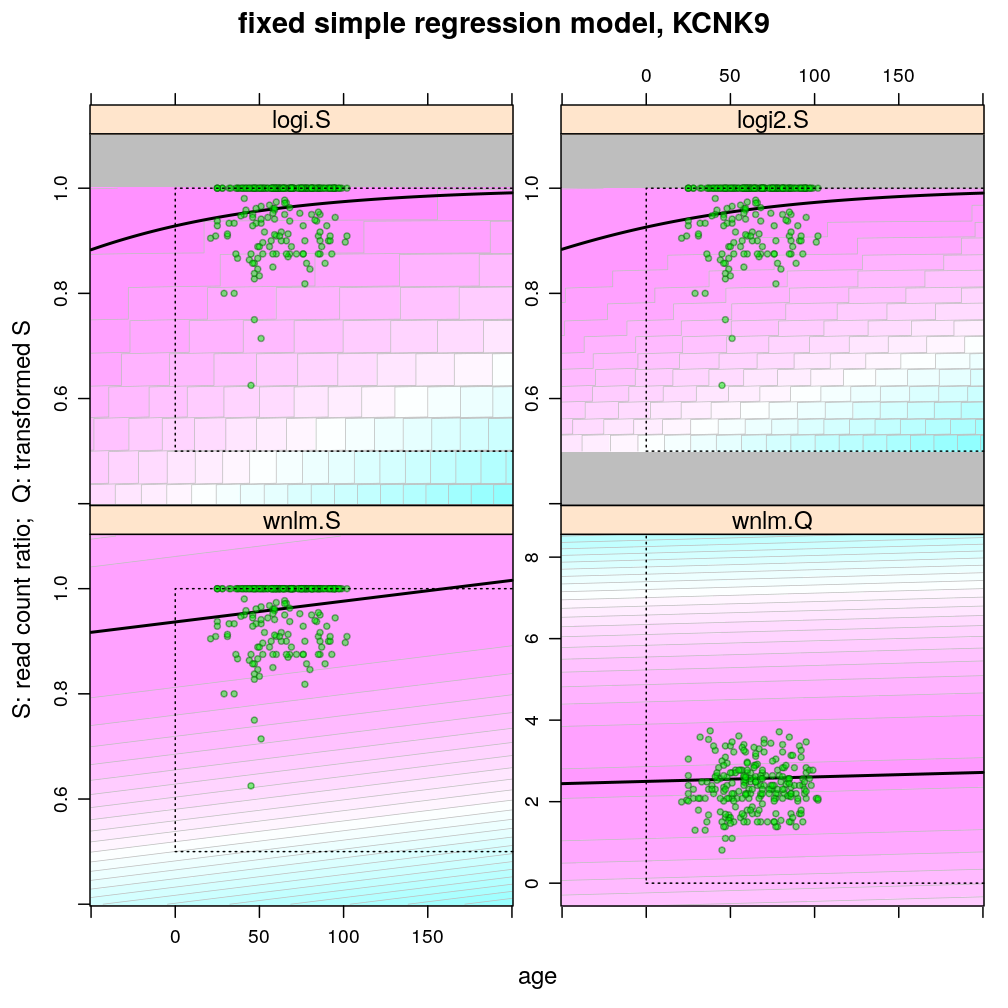
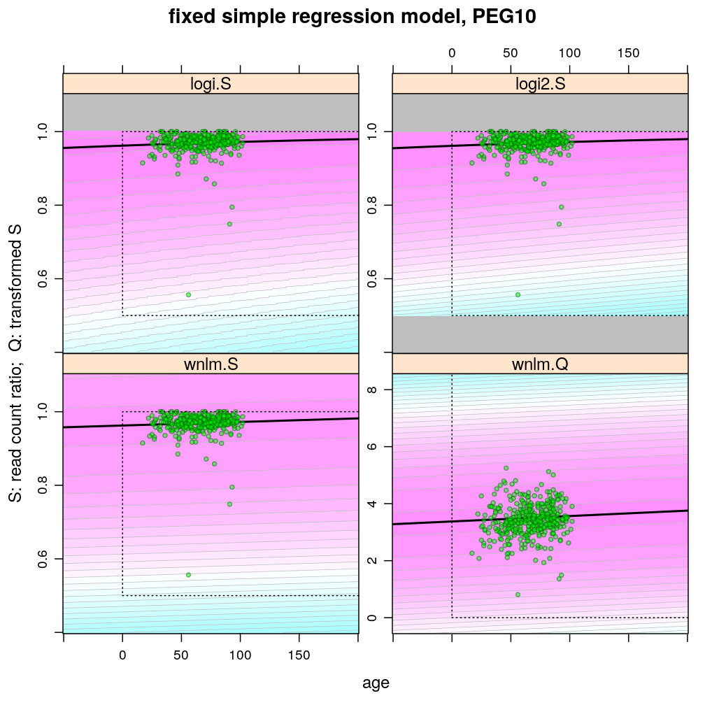
The plots below show the first 4 of the 6 combinations (logi.S, logi2.S, wnlm.S, wnlm.R, unlm.S, unlm.R) of some model family and some response variable ( or ) that were used to fit data. unlm.S and unlm.R are not shown because they are so similar to wnlm.S and wnlm.R, respectively.
For all predicted points of logistic models the total read count (used as the denominator of the binomial error function) was set to be the average of the observed total read counts (given the gene in question).
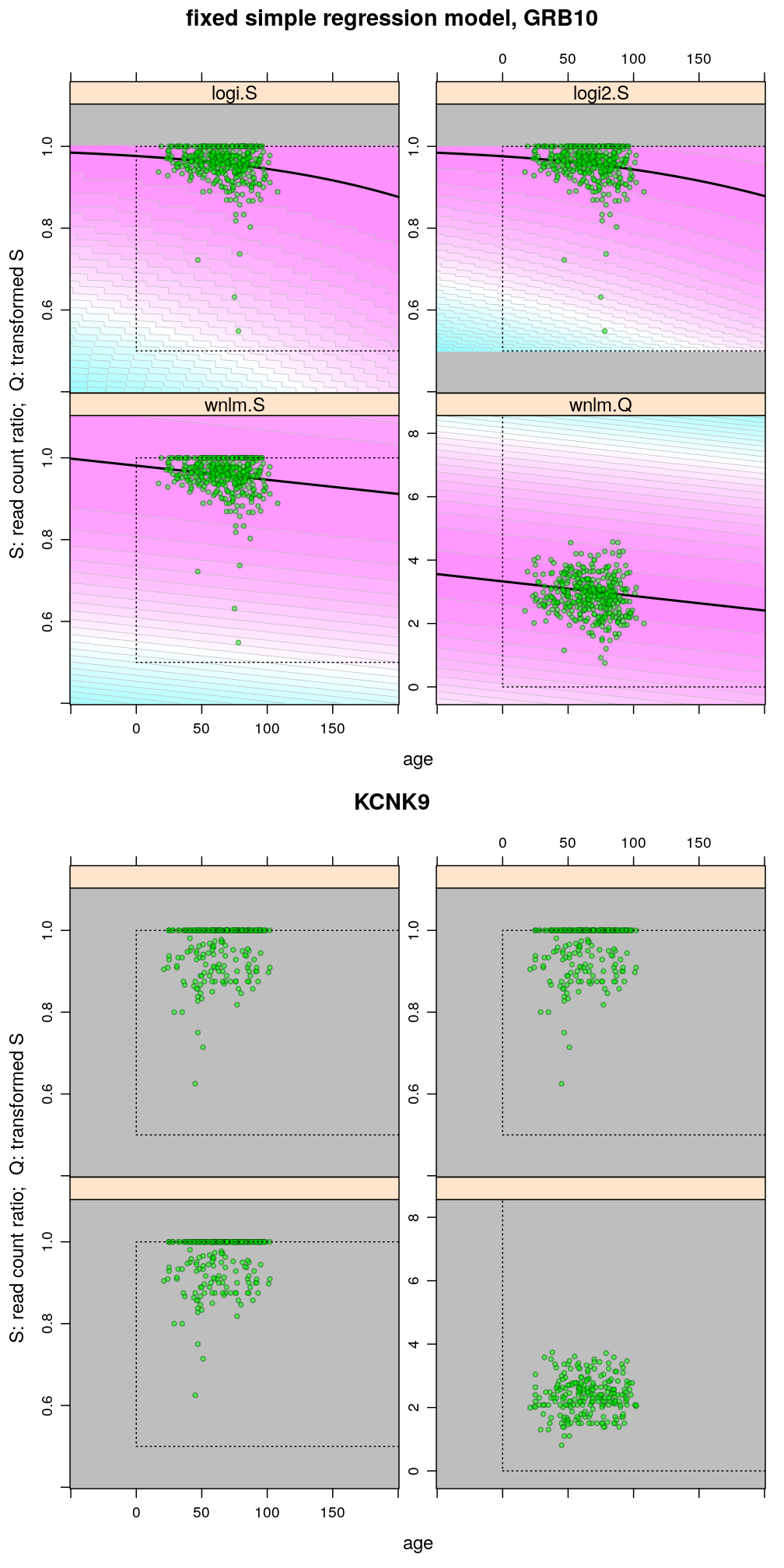
Theoretically possible values (non-negative age and S between 0.5 and 1 or S between 0 and 100) are demarcated by a dotted rectangle. The logi2.S model respects both the upper and lower side of the rectangle but on the lower side it has asymptotically zero variance, which contradicts with the observed large variance of well-balanced (biallelically expressed) genes.
Unlike the normal linear models, both logistic models explain the systematic change of variance with average read count. However, the explained change seems somewhat less than what is observed indicating overdispersion. The weakness of logistic models is that the steepest, most informative, part of their sigmoidal predicted curve lies out of the observed range of data (massive extrapolation).
The rank transformation achieves nearly constant variance allowing a better fit of the normal liear model. But much information is lost in the transformation, which substantially worsens signal-to-noise (explained vs unexplained variance).
gp <-
    lapply(c(GRB10 = "GRB10", ZDBF2 = "ZDBF2", ZNF331 = "ZNF331", KCNK9 = "KCNK9", PEG3 = "PEG3", PEG10 = "PEG10"),
             grid.predictions.1gene)
Examples for down-regulation
Examples for up-regulation
Plot only data
The following plots are generated for overlay with the ones above in presentation slides.
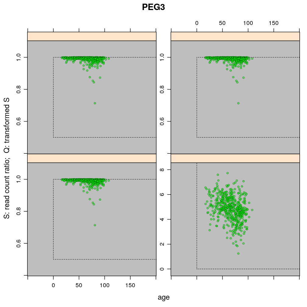
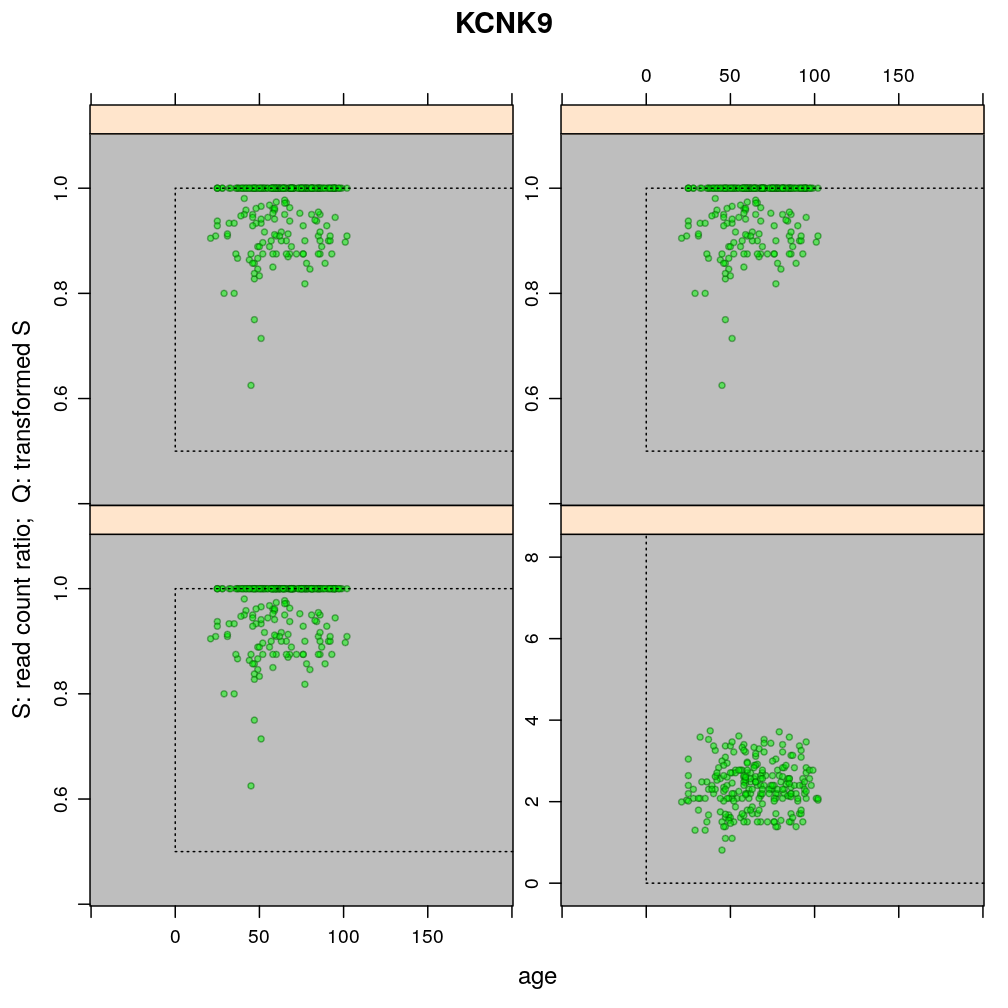
Figure for manuscript
The figures illustrate the widening of prediction intervals under the logistic models but not the normal linear models. The discrete nature of the binomial error distribution under logistic models can also be seen: the denominator of the binomial distribution is 61 (GRB10) and 16 (KCNK9); these were defined as the average of the total read count for a given gene.
print(plots$GRB10, split = c(1, 1, 1, 2), more = TRUE)
print(plots$KCNK9, split = c(1, 2, 1, 2), more = FALSE)
