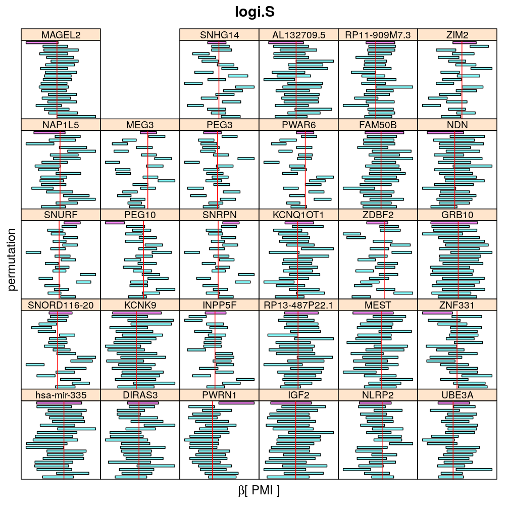
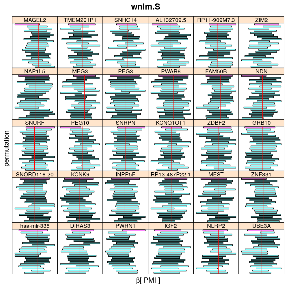
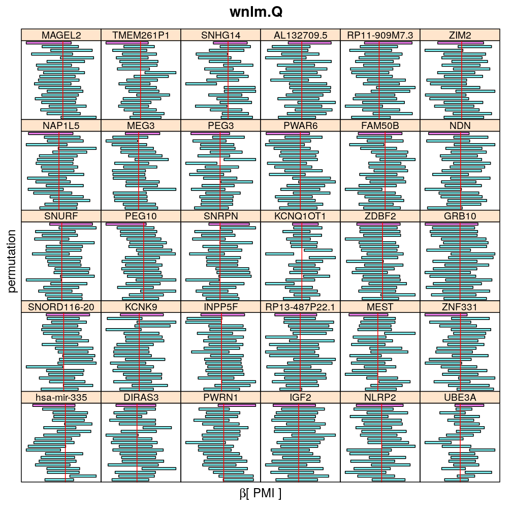
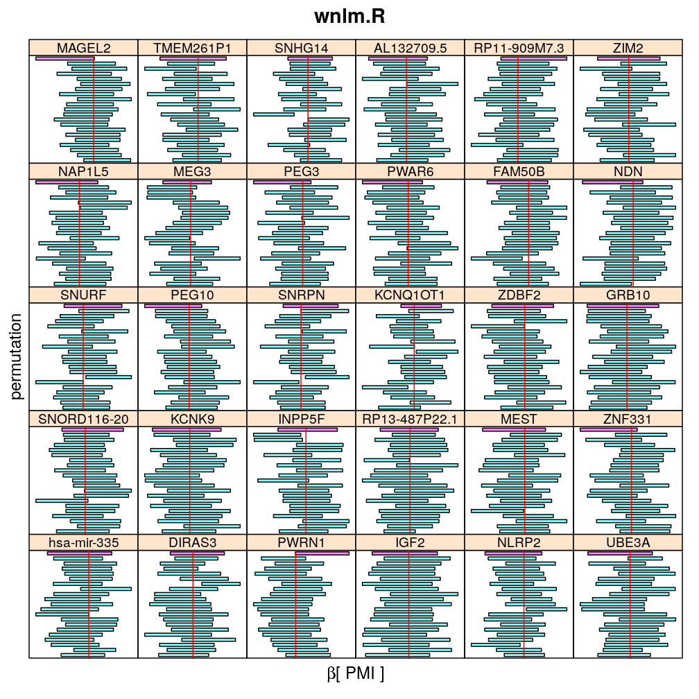
The present analysis investigates more thoroughly the significance of effect on read count ratio of various predictors for various genes. This is done by random permutations of the observed values of any given predictor and fitting the same models to both observed (unpermuted) and permuted data. This approach is thought to provide more accurate p-values and confidence intervals (CIs) than deriving those from only the observed data using the standard way based on normal distribution theory (see ch8.3, p371 in A.C Davison: Statistical Models), which is very sensitive to the quality of model fit. Indeed, a general finding from this analysis is that some genes show more unexpected distribution of CI than others and that variability is explained by diagnostics of model fit for the corresponding genes. See model checking for details.
Introduction
There are several limitations of the (generalized) linear models (e.g. wnlm.R, logi.S) of read count ratio regressed on predictors such as Age, Institution, etc. These limitations might lead to bias in the estimation of regression coefficients , on which some of the main conclusions from this study are based. In particular, a nonzero associated with some predictor indicates either significant effect, or bias. These are only the basic cases; typically we expect to deal with some combination of the two.
The analysis herein aims to distinguish between the two basic cases. This done by randomly re-permuting observations for each predictor (in other words individuals are randomly relabeled for each predictor). Any significant result associated with the permuted predictor must either come from bias or occur “by chance” with probability 1 less the chosen confidence level for .
Calculations
Preparations
## Loading required package: RColorBrewer
##
## Attaching package: 'latticeExtra'
## The following object is masked from 'package:ggplot2':
##
##     layer
Load functions
source("~/projects/monoallelic-brain/src/import-data.R")
source("~/projects/monoallelic-brain/src/fit-glms.R")
source("~/projects/monoallelic-brain/src/graphics.R")
source("2016-09-20-permuted-observations.R")
gene.ids <- unlist(read.csv("../../data/genes.regression.new", as.is = TRUE))
names(gene.ids) <- gene.ids
Get data: observations on predictors (explanatory variables) and on the higher and lower read count from selected genes (more details in a previous post)
E <- get.predictors() # default arguments
Y <- get.readcounts(gene.ids = gene.ids, count.thrs = 0)
Permutations
set.seed(1976)
perm.obs <- sample.int(nrow(E))
names(e.vars) <- e.vars
EP <- lapply(e.vars, function(v) { E1 <- E; E1[[v]] <- E[[v]][perm.obs]; return(E1) })
EP$Unpermuted <- E
set.seed(1976)
perms <- data.frame(cbind(seq_len(nrow(E)), replicate(20, sample.int(nrow(E)))))
names(perms) <- c("U", paste0("P", seq_len(length(perms) - 1)))
Model fitting and CI calculation
# exclude unweighed aggregates UA.8 and UA from fitting
to.fit.ids <- grep("^UA(.8)?$", names(Y), value = TRUE, invert = TRUE)
sel.models <- c("logi.S", "wnlm.Q", "wnlm.R", "wnlm.S"); names(sel.models) <- sel.models
M <- lapply(EP, function(e) do.all.fits(Y[to.fit.ids], G = e, preds = e.vars, sel.models = sel.models))
Betas.Unpermuted <- lapply(M$Unpermuted,
                           function(m) { x <- get.estimate.CI(m); x <- x[ ! x$Coefficient %in% "(Intercept)", ] })
Betas.Unpermuted.95 <- lapply(M$Unpermuted,
                           function(m) { x <- get.estimate.CI(m, conf.lev = 0.95); x <- x[ ! x$Coefficient %in% "(Intercept)", ] })
Betas.Permuted <- lapply(sel.models, get.estimate.CI.permut, M = M, e.v = e.vars, conf.lev = 0.99)
Betas.Permuted.95 <- lapply(sel.models, get.estimate.CI.permut, M = M, e.v = e.vars, conf.lev = 0.95)
Betas <- aggregate.CI.permut2(perms = perms, gene.ids = gene.ids, e.vars = e.vars,
                              sel.models = sel.models, E = E, Y = Y[gene.ids], conf.lev=0.99)
Results
Single permutation
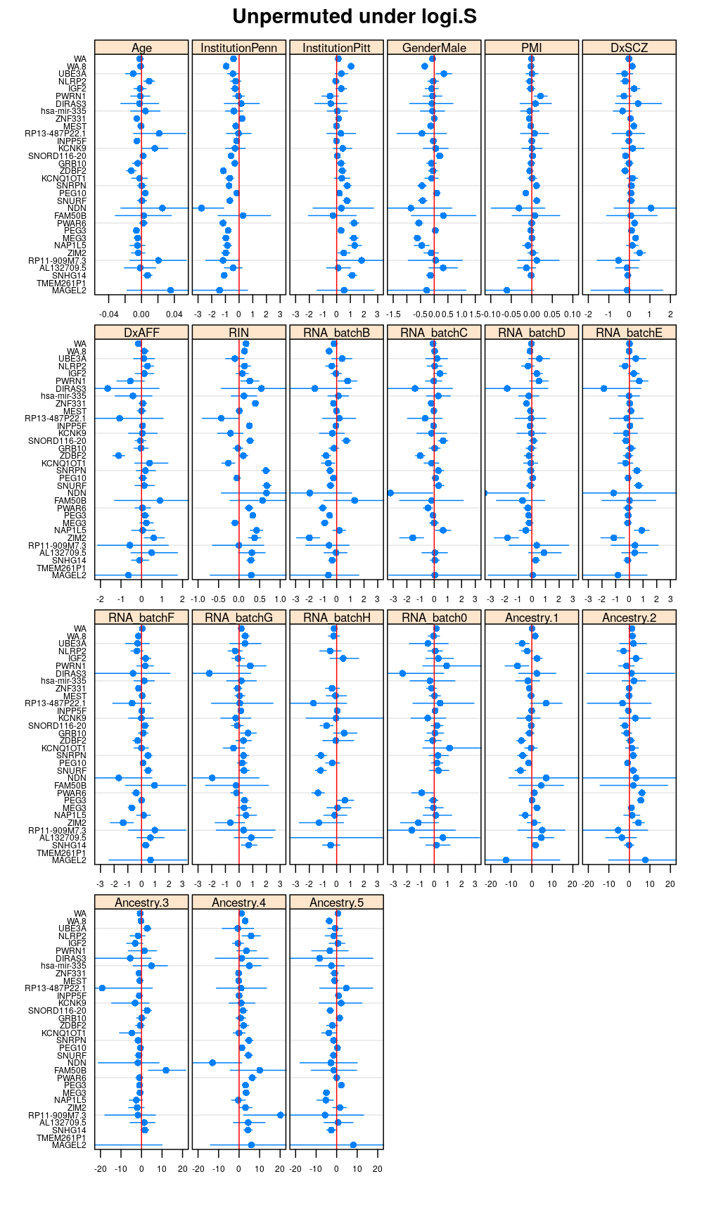
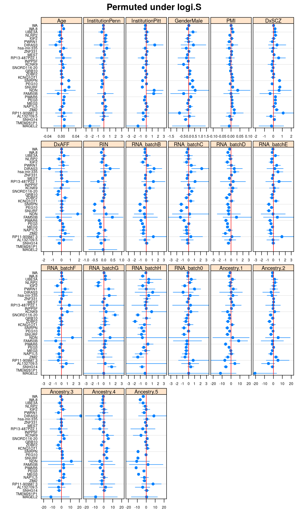
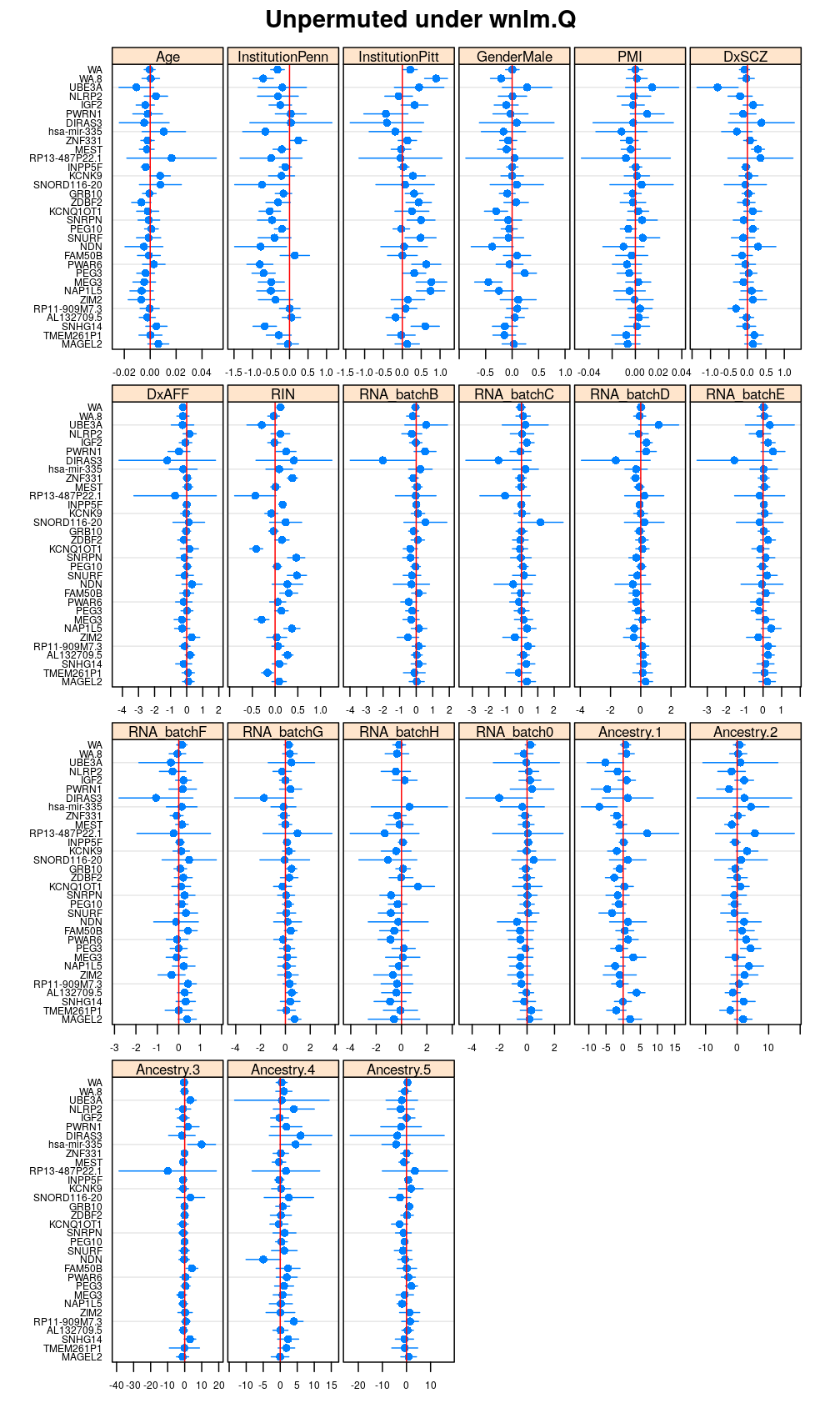
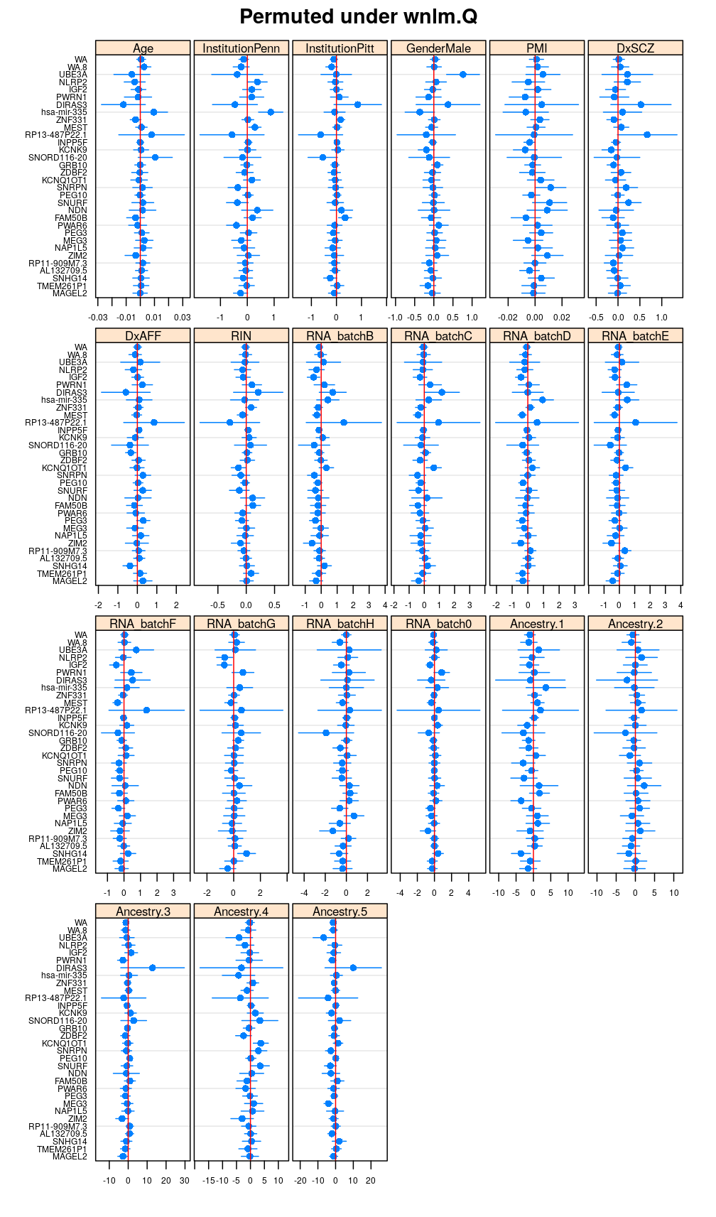
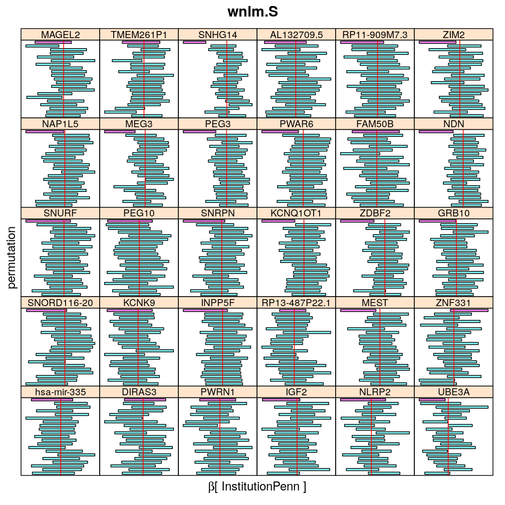
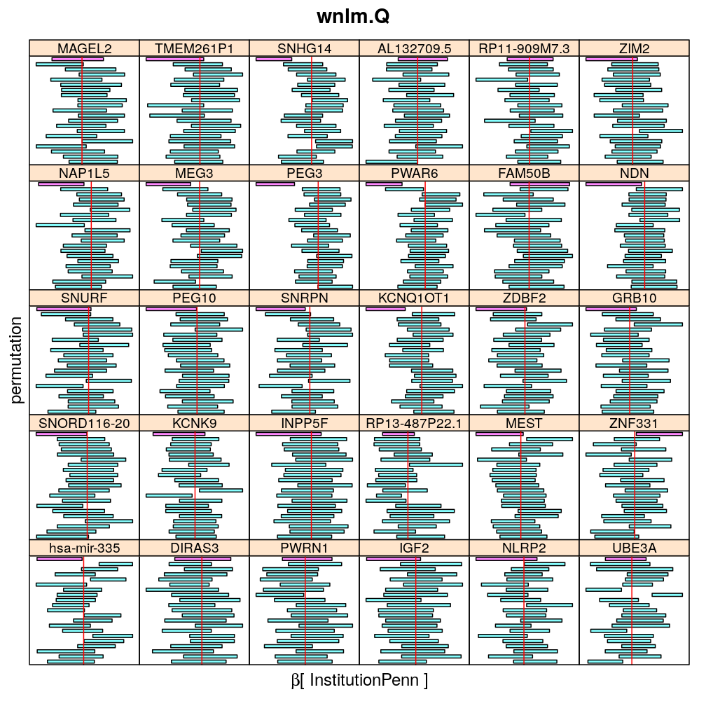
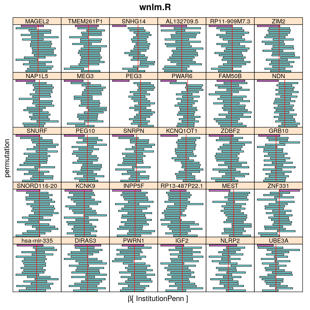
Both the unpermuted and permuted data was fit by the models logi.S, wnlm.Q, wnlm.R, wnlm.S. Given the poor fit for wnlm.S and the relatively low power of wnlm.R only wnlm.Q and logi.S associated results are presented in the following four plots. These results are the estimates and CI for at confidence level of . The following observations and conclusions may be noted:
Under wnlm.Q there are 59 significant coefficients before and 37 after permutation. In contrast, under logi.S there are 185 and 191 (before and after). But taking only those coefficients that are significant under both models yields 44 and 27 (before and after, respectively).
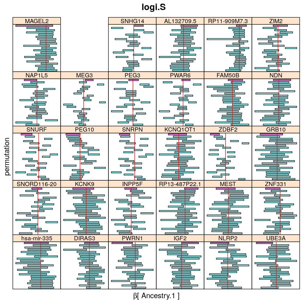
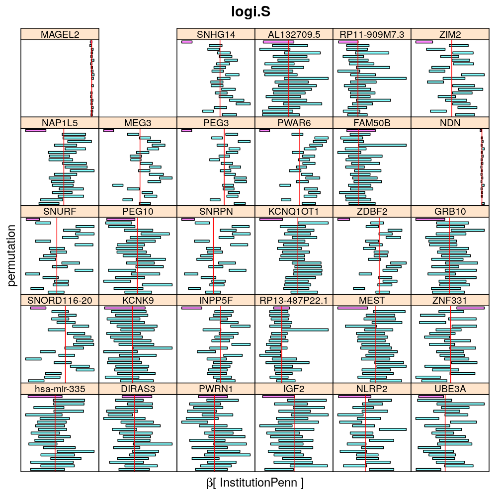
Under logi.S the following pattern is observed. For some genes (e.g. GRB10, ZDBF2) permutation tends to abolish significance—if observed—, whereas for other genes (e.g. SNRPN, SNURF) there are many significant coefficients after permutation. This suggests systematic differences between genes: better fit of logi.S to the data for the former set of genes and poorer for the latter gene set. The poor fit explains the many significant coefficients after permutation.
my.segplot(data = Betas.Unpermuted$logi.S, xlim = my.xlim, main = "Unpermuted under logi.S")
Repeated permutations
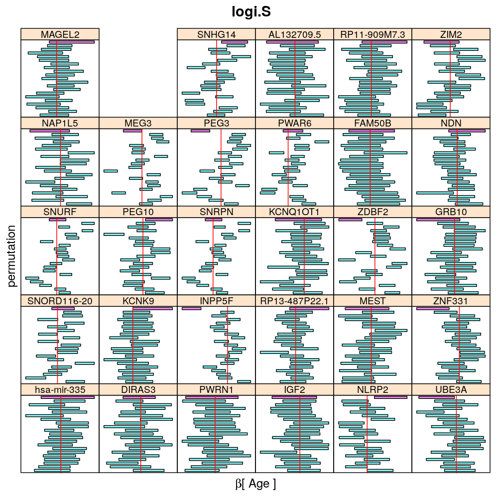
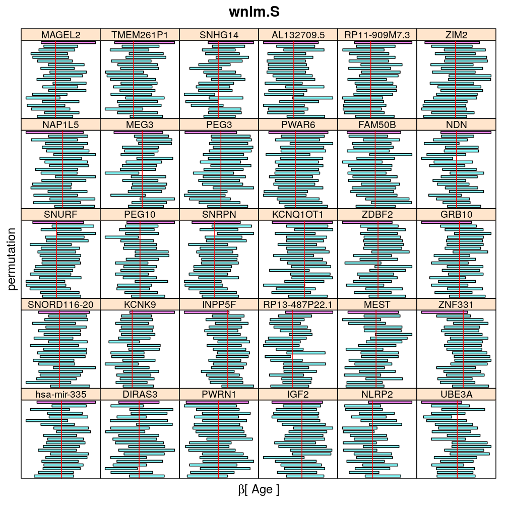
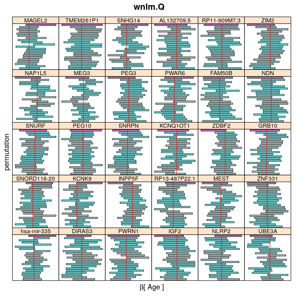
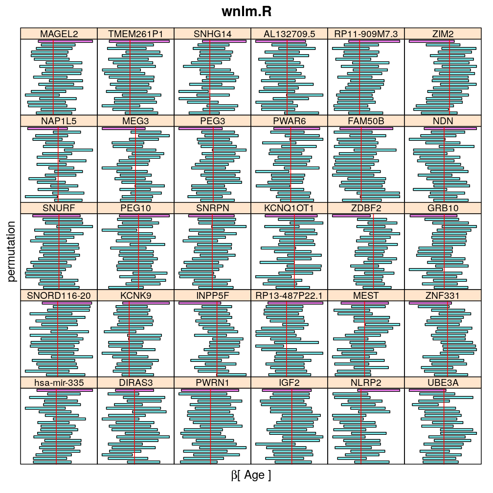
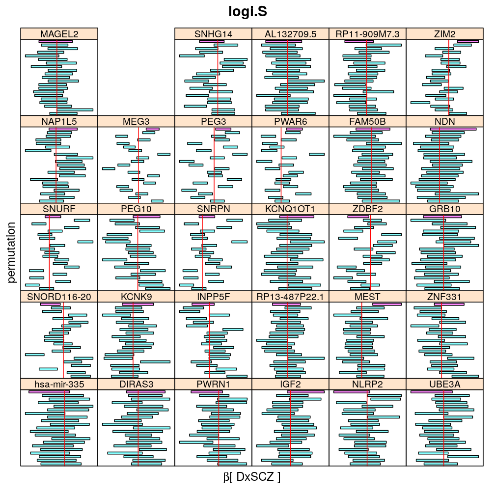
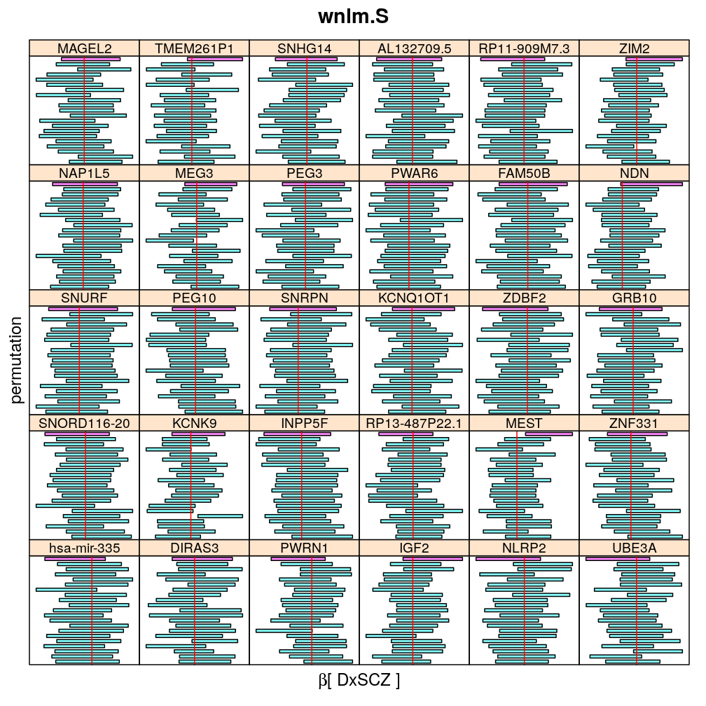
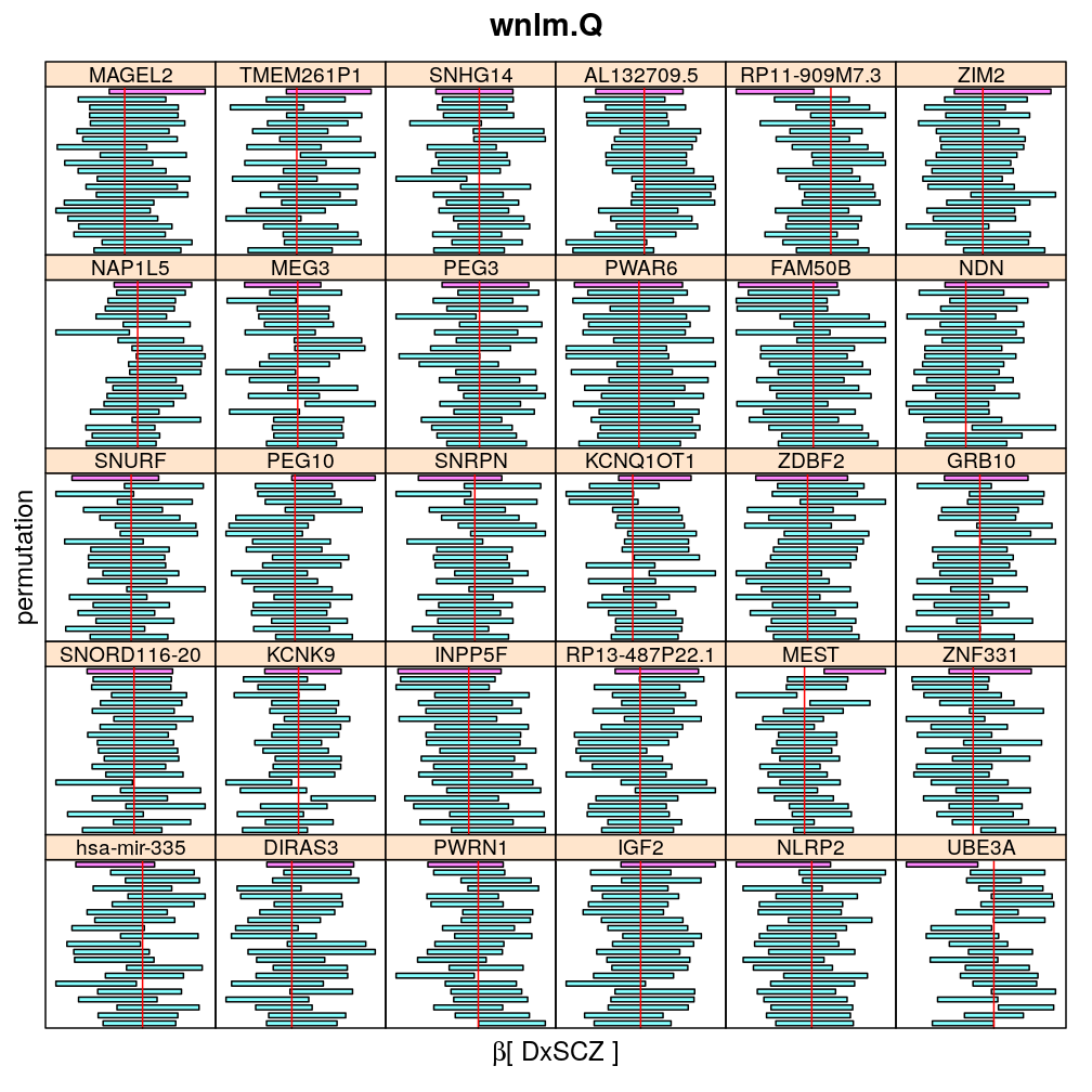
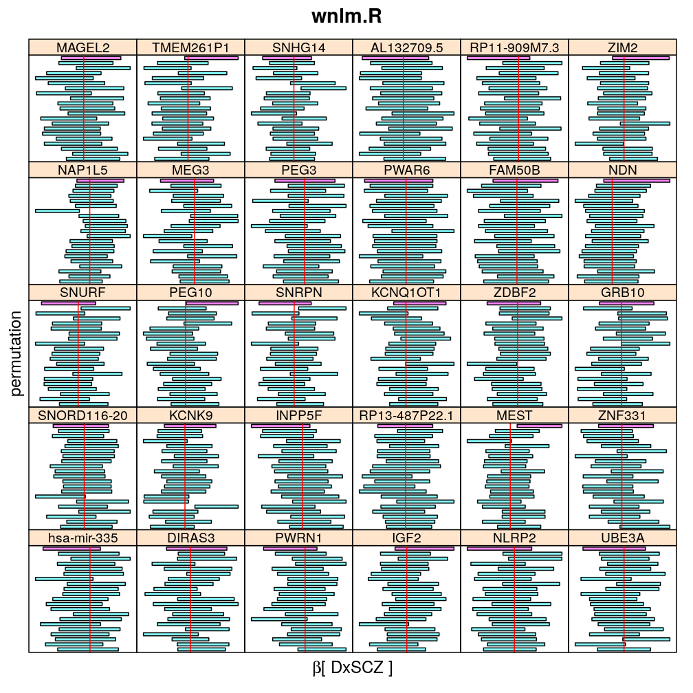
The above analysis is extended now in two ways: presenting CI for several, though not all, with
- 20 random permutations
- under all selected models logi.S, wnlm.Q, wnlm.R, wnlm.S
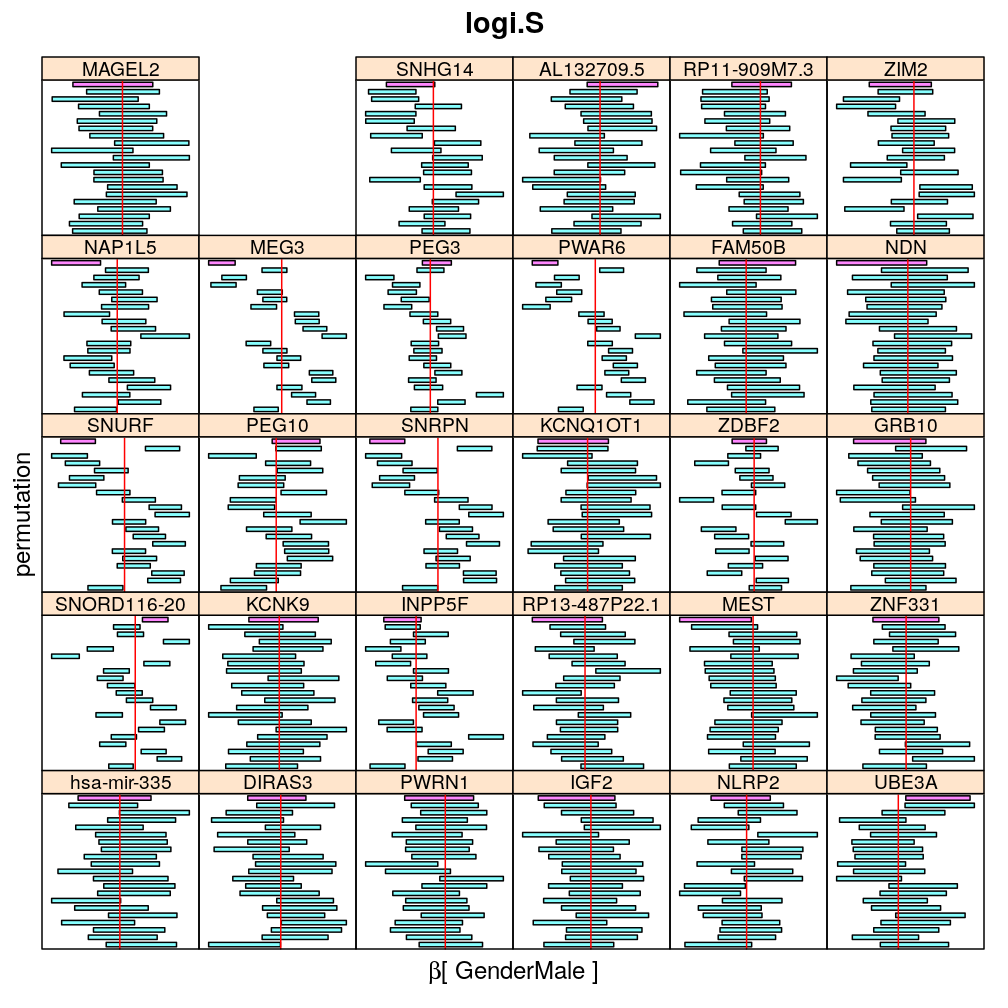
Note that genes (panels) are skipped for which the fit did not converge. In the present analysis this applies only to logistic models, since those employ iterative least squares algorithm. Normal linear models, on the other hand, use a one-step least square algorithm and thus are guaranteed to “converge”.
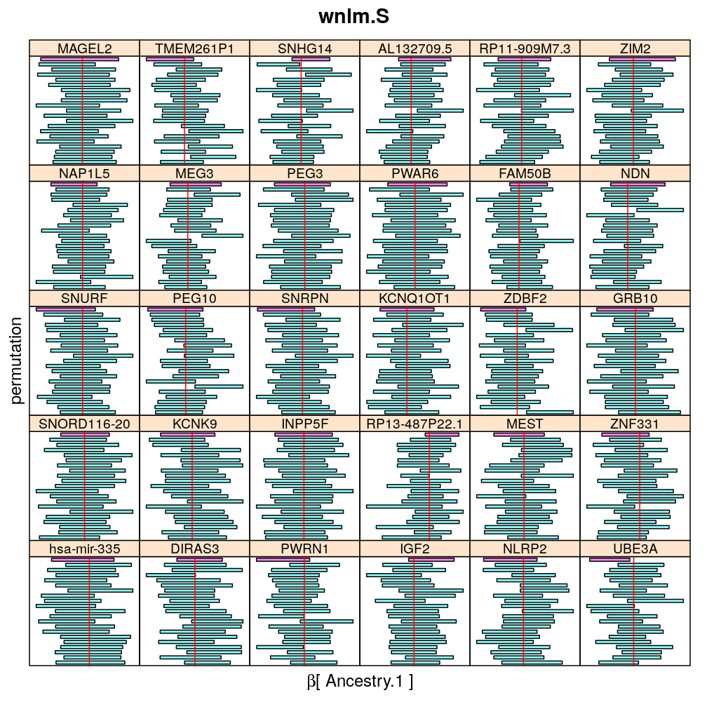
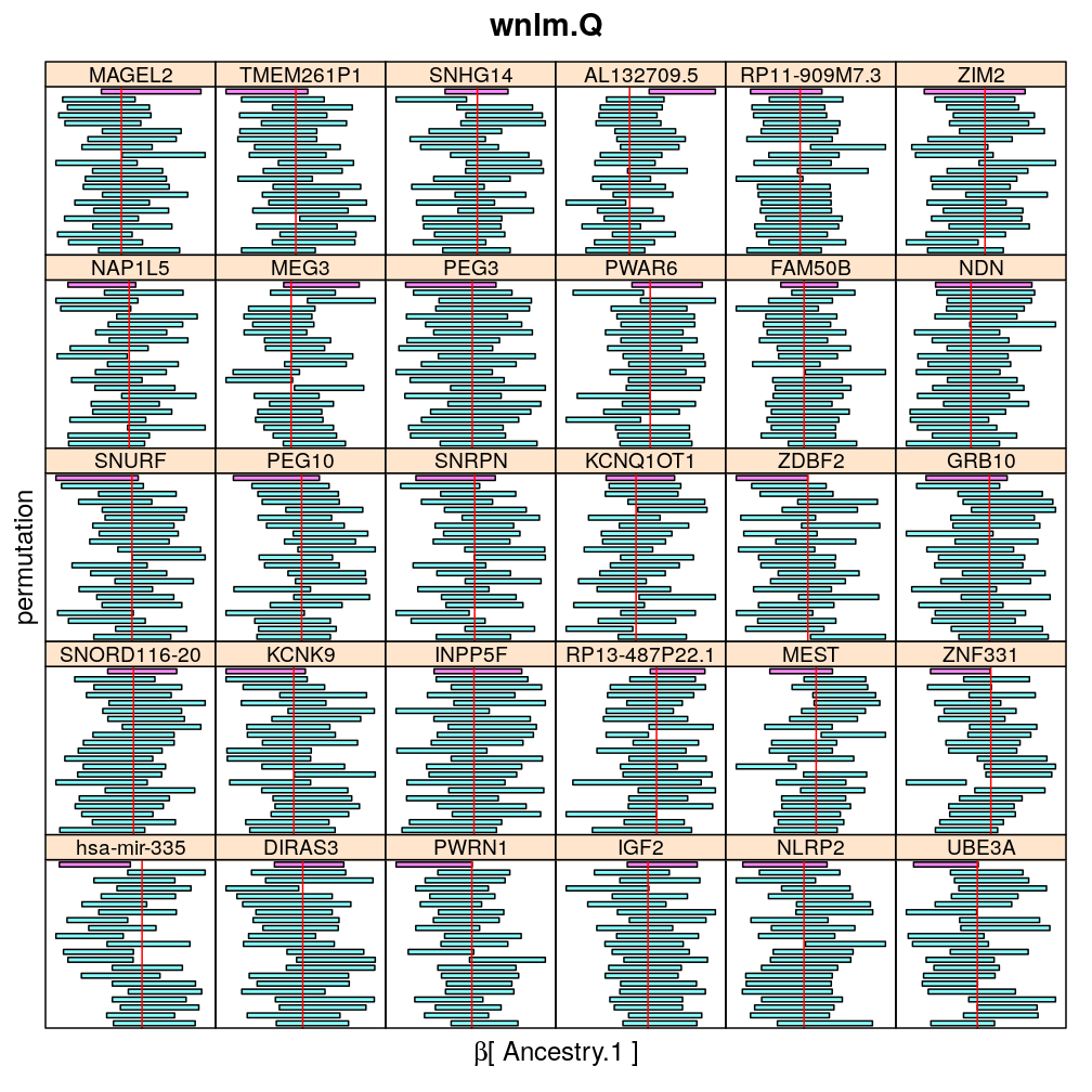
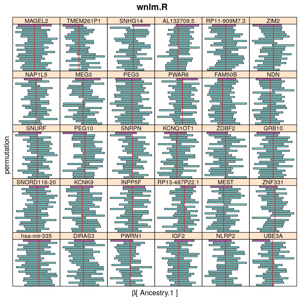
The following general results emerge from the following plots
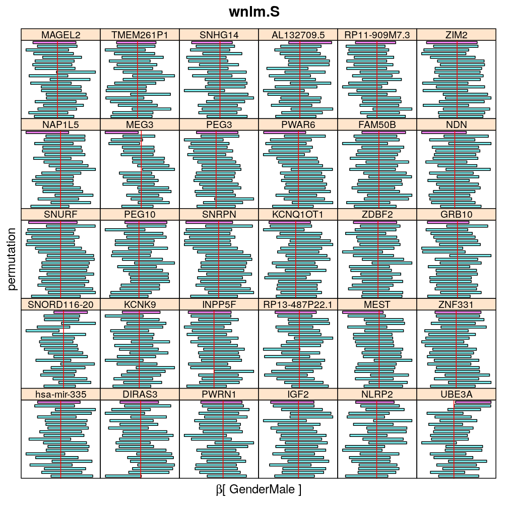
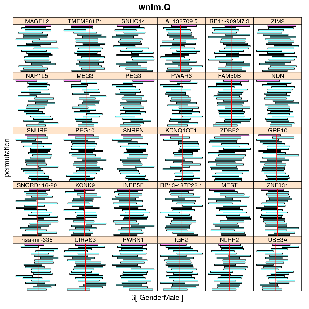
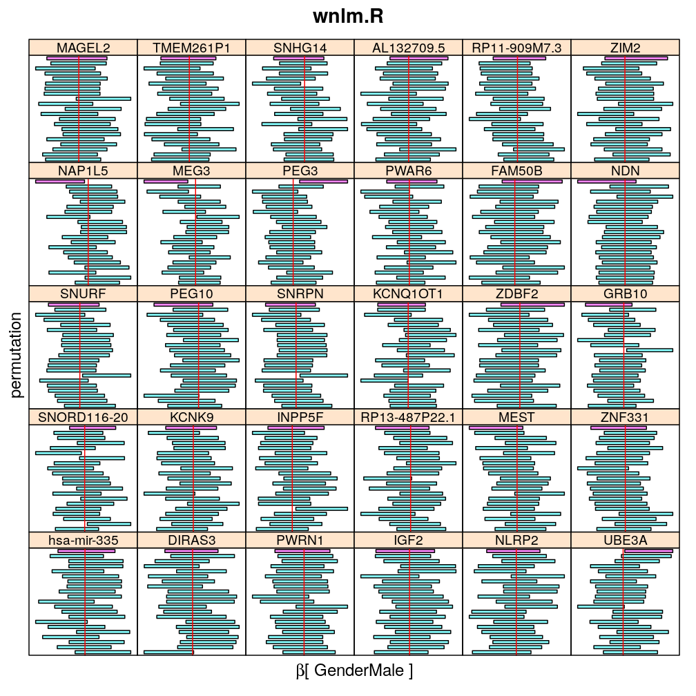
- in general the distribution of permuted CI tends to be wider than expected
- at 99 % confidence level only CI per gene per model is expected to fall out side the zero line but the observations show a greater number of such CIs
- the distribution of permuted CI varies greatly both across models and genes
- under wnlm.Q and wnlm.R the distributions of CI are somewhat closer to the expected ones than under logi.S
- the various models tend to agree qualitatively
- therefore it is beneficial to use a consensus approach by defining significance that is fulfilled both under wnlm.Q and logi.S
- poorly fit genes tend to show greater departure from the expected CI distribution (cf. model checking analyses)
Age
# skip genes for which the fit did not converge
# applies to logistic models, since those employ iterative least squares algorithm
# normal linear models use a one-step least square algorithm and thus are guaranteed to "converge"
skip <- ! sapply(M$Unpermuted$logi.S, `[[`, "converged")[1:30]
my.segplot2("Age", "logi.S", skip = skip) # fit has not converged for gene ranked 2 (TMEM261P1)
Gender
Dx
Ancestry
Institution
PMI
