Lab Notebook

The present article extends previous inference of regression parameters $\beta$ (see extending ANOVA) with a conditional analysis. Operationally, conditioning takes a subset of all observations (i.e. individuals/RNA preparations) defined by a condition. In the present, rather special, case a condition is defined by a single level of a single factor-type (i.e. categorical) predictor/explanatory variable. However, more general conditioning setups could also be explored. In that case multiple predictors might be selected, of which some might be continuous (i.e. a covariate) while others categorical, and for each predictor a possibly compound event (e.g. multiple levels of a factor) might be taken.

The choice of Institution and Gender as selected predictors for conditioning is motivated by the fact that they are categorical with 3 and 2 levels, respectively, and that they are clearly associated with Age (see “scatter plot matrices” in this article).

Preparations

Load libraries and my custom functions.

library(lattice)
library(latticeExtra)

## Loading required package: RColorBrewer

source("~/projects/monoallelic-brain/src/import-data.R")
source("~/projects/monoallelic-brain/src/fit-glms.R")

Next:

1. import data
2. create subsets (conditioning)
3. fit models (logi.S, wnlm.Q)
4. calculate confidence intervals (CI)

E <- get.predictors() # default arguments
# updated gene set
gene.ids <- unlist(read.csv("../../data/genes.regression.new", as.is = TRUE))
names(gene.ids) <- gene.ids
Y <- get.readcounts(gene.ids = gene.ids, count.thrs = 0)
# predictors for conditioning
s.p <- c("Institution", "Gender")
# exclude unweighed aggregates UA.8 and UA from fitting
Z <- Y[grep("^UA(.8)?$", names(Y), value = TRUE, invert = TRUE)]
M <- list(logi.S = l.l.do.all.fits.sset(s.p, Z, E, e.vars, "logi.S"),
          wnlm.Q = l.l.do.all.fits.sset(s.p, Z, E, e.vars, "wnlm.Q"))
# regression coefficients: estimates and CI at 99 % level
Betas <- lapply(M, function(l3m) {
    df <- do.call(make.groups,
                  lapply(l3m,
                         function(l2m)
                             do.call(make.groups,
                                     lapply(l2m,
                                            get.estimate.CI, conf.lev = 0.99))))
    names(df)[-(1:5)] <- c("Level", "Cond.Var")
    return(df)
})

Results

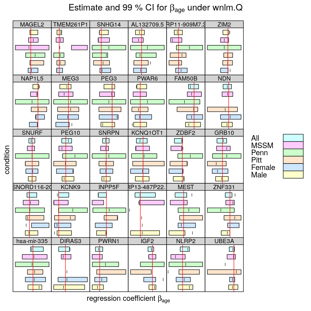
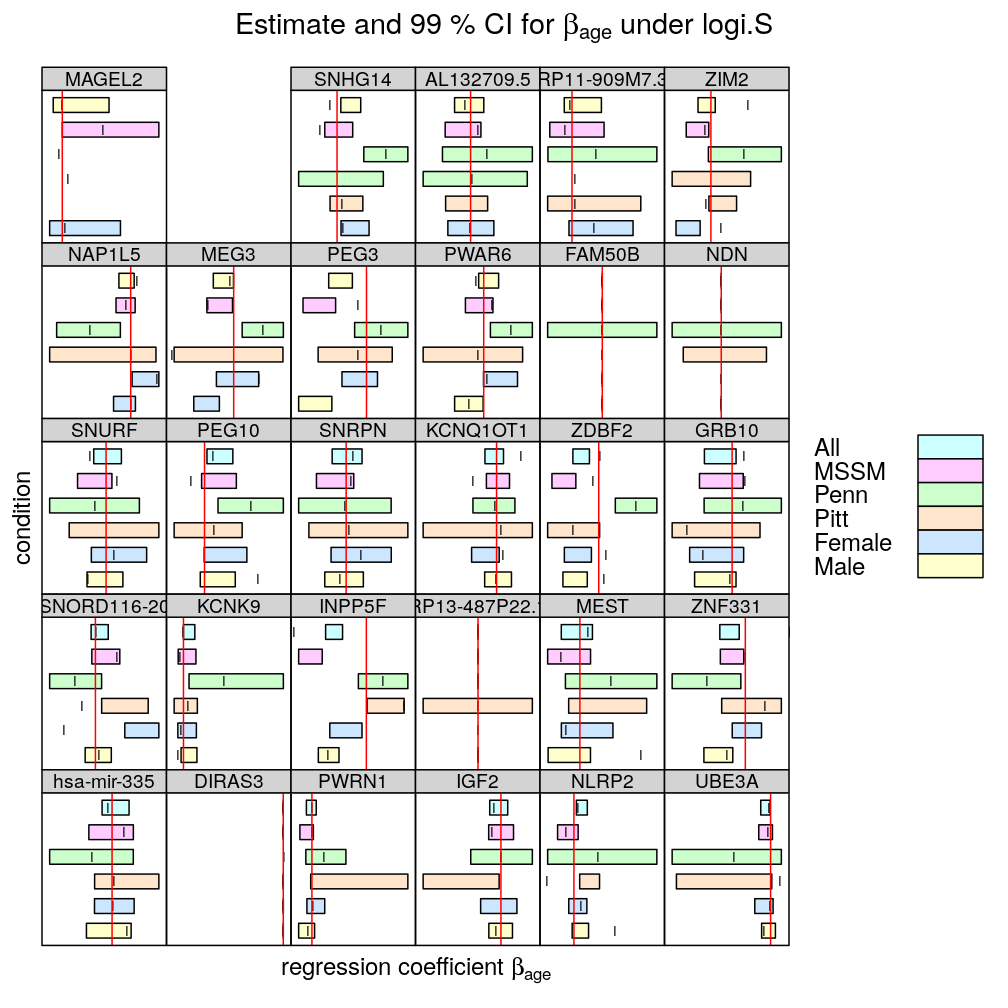
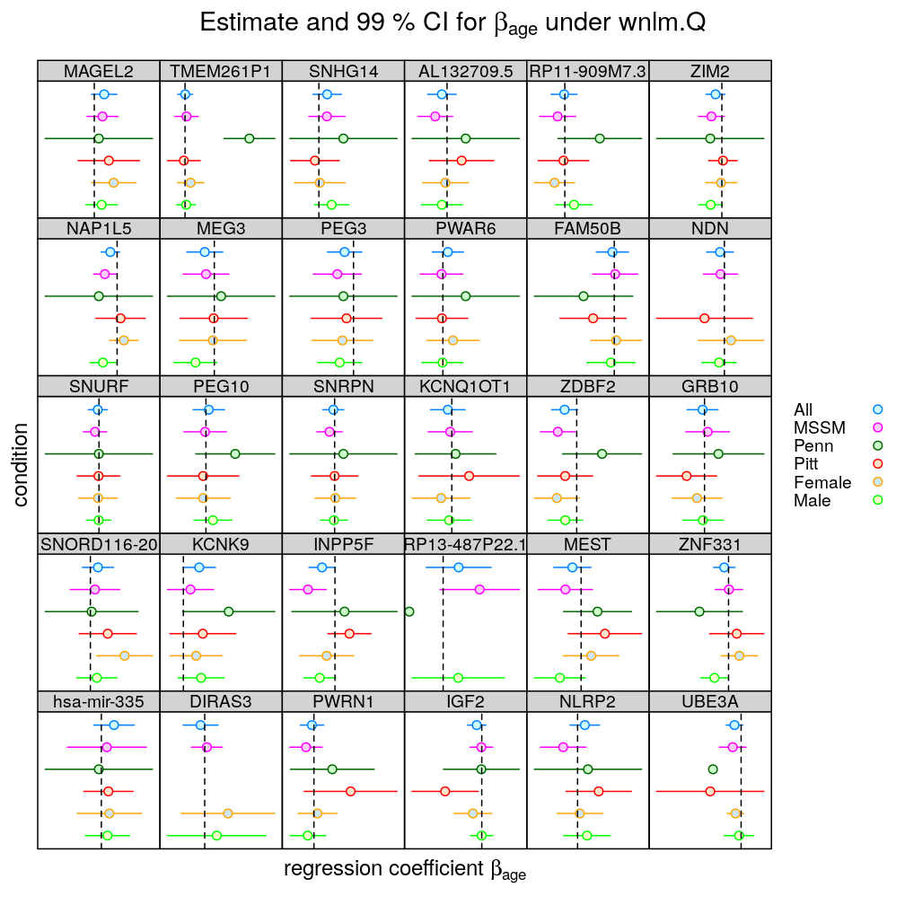
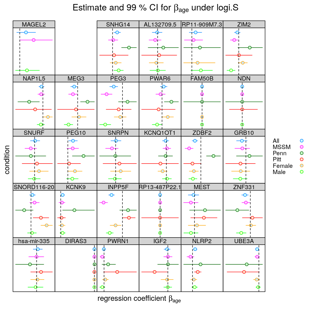
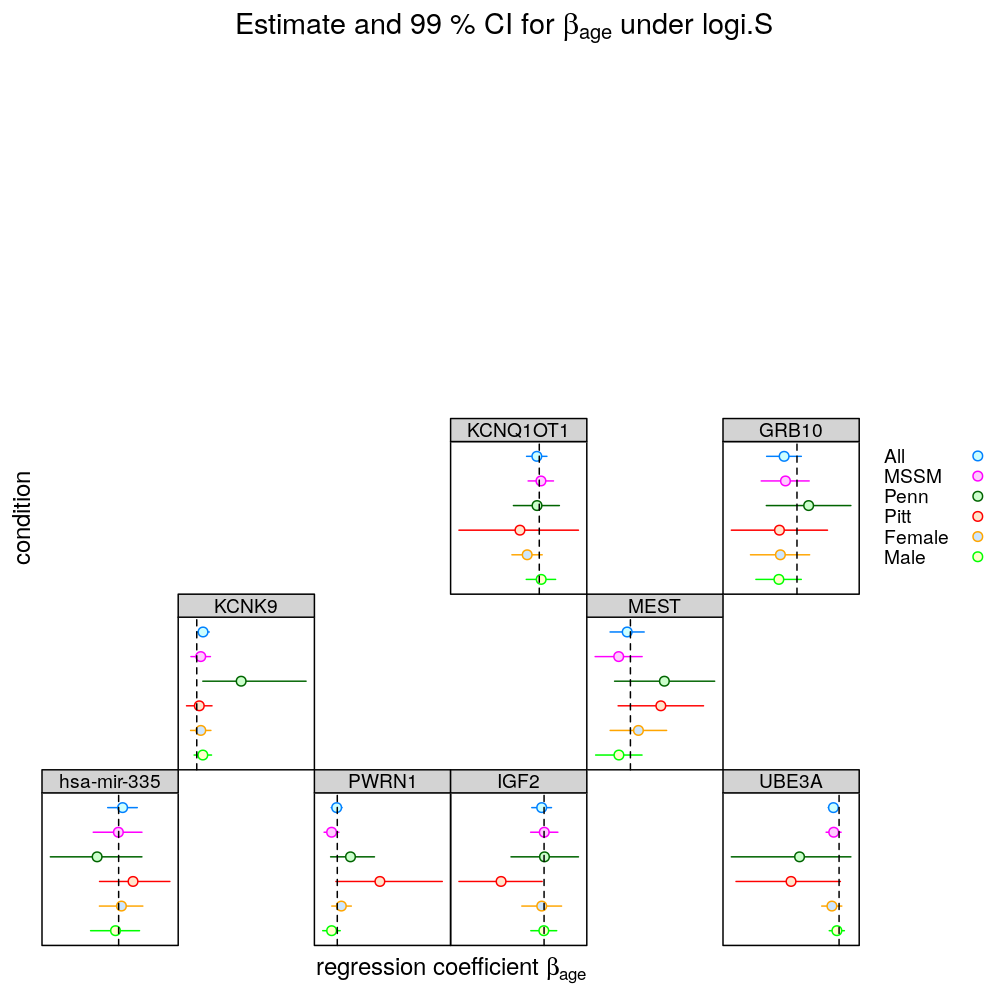
In the following plots the effect of 5 conditions (MSSM, …, Female) is explored on the inferred $\beta_\mathrm{age}$. All denotes the full set of observations (no conditioning), as done before. Note the following

• two types of regression model were fitted
  • logi.S: logistic model fitted to untransformed $S$
  • wnlm.Q: weighted normal linear model fitted to quasi-log-transformed $S$
• the colored bars show confidence intervals (CI) for $\beta_\mathrm{age}$
  • some CI are missing (could not be calculated because of too little variance in the response)
• the vertical red line spanning each graph is at $\beta = 0$, so when a CI does not “cross” that line we can conclude that the effect of Age is significant on the response ($p < 0.01$)
• the vertical notch “I” inside the bars marks the least square estimate $\hat{\beta}_\mathrm{age}$
• the individual displays (each corresponding to a given gene or aggregate dataset across genes) are scaled differently to emphasize the effects of conditioning.
• the fit for TMEM261P1 did not converge under logi.S so the results are missing; for consistency TMEM261P1 is excluded for wnlm.Q as well

The same results plotted with different style

For presentations

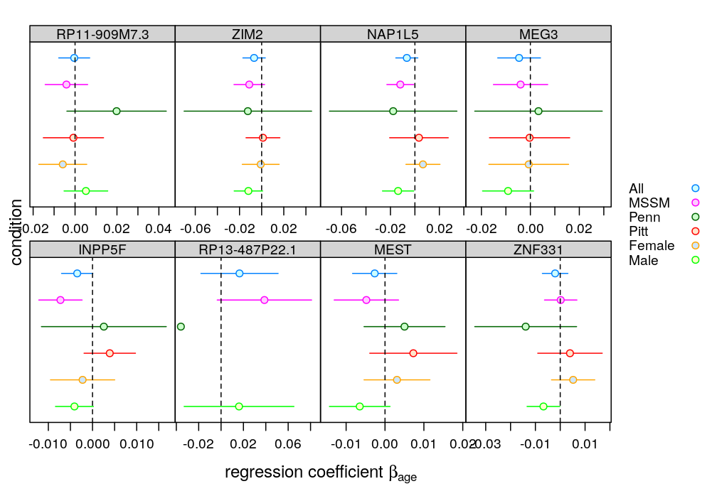
Exclude those genes for which the fit was deemed insufficient. Requires the file model-checking.csv, which was generated in a subsequent analysis.

Conclusion

The main results and their interpretation can be summarized as follows:

• For several genes conditioning qualitatively changes the effect of Age on the response in a pattern that is similar under logi.S and wnlm.Q. This suggests that some assumption(s) that is shared by both models is violated. The most obvious shared assumption is linearity. In other words, (generalized) linear models fail to capture the complex dependency structure that relates predictors to each other and to the response. Bayesian networks provide the most general framework suitable to deal with such dependency structure. A less general alternative is using (generalized) linear models extended with interaction terms.
• Under wnlm.Q conditioning has weaker effect than under logi.S. This suggests that while logi.S is more powerful than wnlm.Q (as expected from a theory-based weighting scheme) it is also less robust for reasons extraneous to nonlinearity. A logi.S-specific assumption is the sigmoidal link function (logistic function), whose inflection point is well beyond several hundred years for all genes and thus far beyond the range of Age data. This need for extrapolation makes logi.S particularly sensitive to outliers, which is worsened by the reduction of the number of observations. That adverse effect is stronger in the case of conditioning on Penn or Pitt than on MSSM, which alone provided $\approx 55 \%$ of the observations. Consistent with this, conditioning on MSSM has the smallest effect. Another potential limitation of the logi.S model is the assumption that the error distribution is binomial (see discussion on overdispersion in the voom paper).
• Conditioning on the Penn or Pitt levels of Institution has in general larger effect than that on levels of Gender. This is consistent with the stronger association of Age to Institution than to Gender, found previously.

How to deal with the present limitations?

Suggested alternatives, roughly in increasing model complexity

1. under the present models interpret the results more carefully
   • pro: no further analysis required
   • con: the conclusion that age has effect on allelic imbalance remains weakly established
2. linear modeling with voom/limma
   • pro: (1) allows fitting normal linear models on suitably transformed $S$ with the advantage of more power than wnlm.Q and (expectedly) more robustness to nonlinearity than logi.S; also (2), voom/limma uses a more detailed form of data, at the level of SNPs instead of genes, potentially using available information more efficiently; (3) mature R packages are available
   • con: substantial additional analysis, including the recovery of the full (i.e. SNP-based) read count data
3. extend present models with interaction terms such as that between Age and Institution
   • pro: can be performed on the readily available gene-based read count data
   • con: including too few interactions may not suffice correcting for nonlinearity whereas even a few interaction terms greatly increase the number of parameters, resulting in overfitting, therefore this approach might need to be combined with formal model selection implemented in for instance the stats package of R (see add1 and step functions) to find the best balance between model fit and parsimony
4. use Bayesian networks (BN)
   • pro: even the most complex dependency structure can be captured by a BN
   • con: many details of statistics and software implementation must be worked out