Permutation Test

This analysis extends permuted observations to testing hypotheses $\beta_j=0, \; j=1,...,p$ for any gene. This is done by random permutation tests, which provide only approximate p-values in contrast with exact permutation tests (which are unpractical in the present case due to the large number $n!$ of all permutations of $n\approx 500$ cases). These approximations more or less agree with the “theoretical” p-values, which are based on the hypothesis that the Studentized $\hat{\beta}_j$ follows a t-distribution on $n - p$ degrees of freedom (see ch8.3, p371 in A.C Davison: Statistical Models):

$\begin{equation} \frac{\hat{\beta}_j - \beta_j}{\sqrt{S^2 \left[ (X^\top X)^{-1} \right]_{jj}}} \sim t_{n - p}, \end{equation}$

where $S^2$ is the unbiased estimate of the error variance (based on the residual sum of squares), and $X$ is the design matrix.

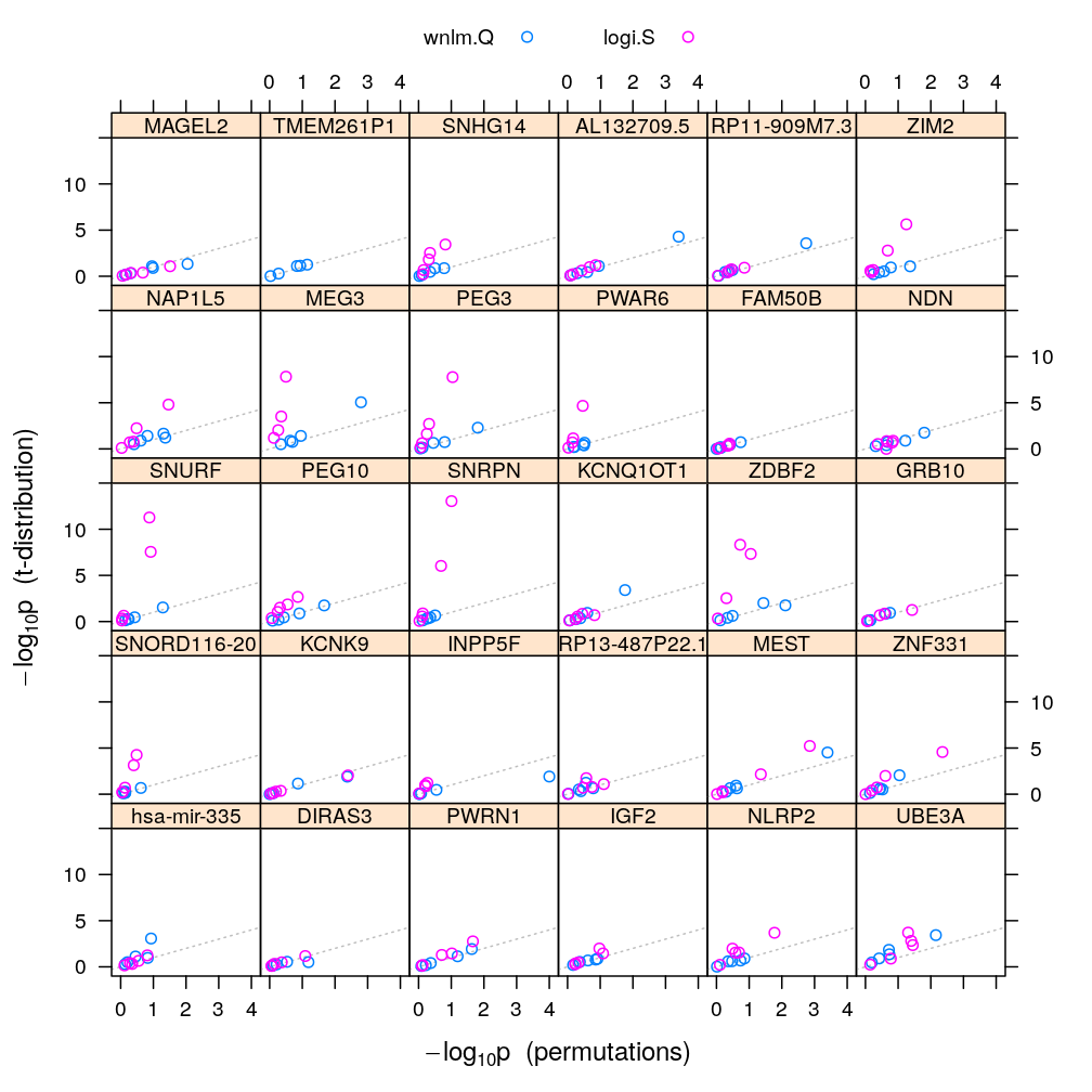
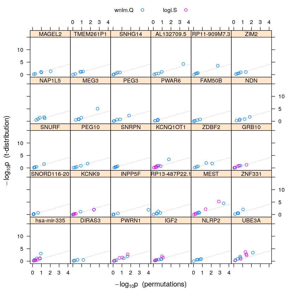
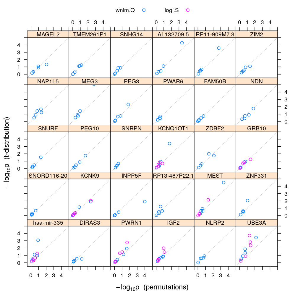
The t-distribution comes from the second order assumptions on the error $\epsilon_i$ and on their normality; from these the normality of the residuals $e_i$ follows. Thus normality of $e_i$ is a prerequisite for deriving p-values using the above theoretical approach. In agreement with this comparison to the model checking results, in particular the normal Q-Q plots of residuals, reveals that the two approaches to p-value calculation agree as long as the model fits the data well. Otherwise the t-distribution based approach tends to produce much lower p-values and therefore exaggerate the significance that $\beta_j\neq 0$ , as seen for several “poorly-fit” genes under the logistic model logi.S.

Click regr-coefs.csv (long format) and regr-coefs-w.csv (wide format, annotated with stars) to download the saved csv files reporting both p-values and the estimate for all regression coefficients. Click signif-gene-effects-wnlm.Q.csv, signif-gene-effects-logi.S.csv, signif-gene-effects-either.csv, or signif-gene-effects-both.csv for a gene-centric list of significant coefficient–gene associations mediating various biological effects, where each list corresponds to a rule of aggregation of p-values across the wnlm.Q and logi.S model types. For the corresponding coefficient centric lists see signif-effect-genes-wnlm.Q.csv, signif-effect-genes-logi.S.csv, signif-effect-genes-either.csv, or signif-effect-genes-both.csv.

Preparations

## Loading required package: RColorBrewer

## 
## Attaching package: 'latticeExtra'

## The following object is masked from 'package:ggplot2':
## 
##     layer

Load functions

source("~/projects/monoallelic-brain/src/import-data.R")
source("~/projects/monoallelic-brain/src/fit-glms.R")
source("~/projects/monoallelic-brain/src/graphics.R")

gene.ids <- unlist(read.csv("../../data/genes.regression.new", as.is = TRUE))
names(gene.ids) <- gene.ids
names(e.vars) <- e.vars

E <- get.predictors() # default arguments
Y <- get.readcounts(gene.ids = gene.ids, count.thrs = 0)

set.seed(1976)
perms <- data.frame(cbind(seq_len(nrow(E)), replicate(n.perm <- 1e4, sample.int(nrow(E)))))
names(perms) <- c("U", paste0("P", seq_len(n.perm)))
sel.models <- c("wnlm.Q", "logi.S")
sel.vars <- e.vars[c(1, 3, 5, 8)]
system.time(Betas <- aggregate.CI.permut2(perms = perms, gene.ids = gene.ids, e.vars = e.vars,
                                          sel.vars = sel.vars, sel.models = sel.models,
                                          E = E, Y = Y[gene.ids], skip.CI = TRUE))

##      user    system   elapsed 
## 18748.892     5.076 18754.811

Results

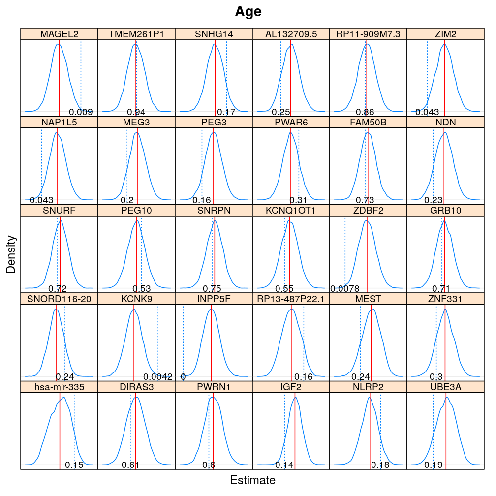
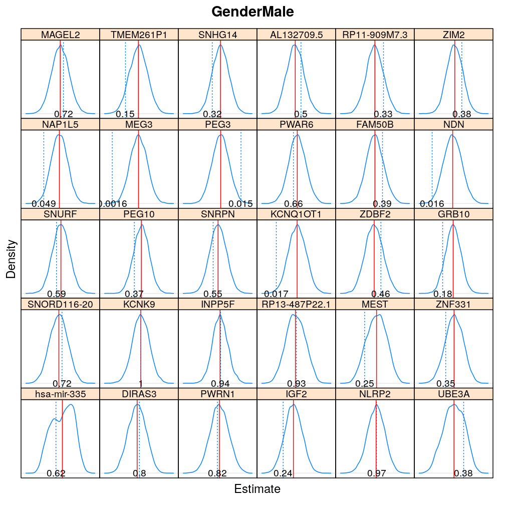
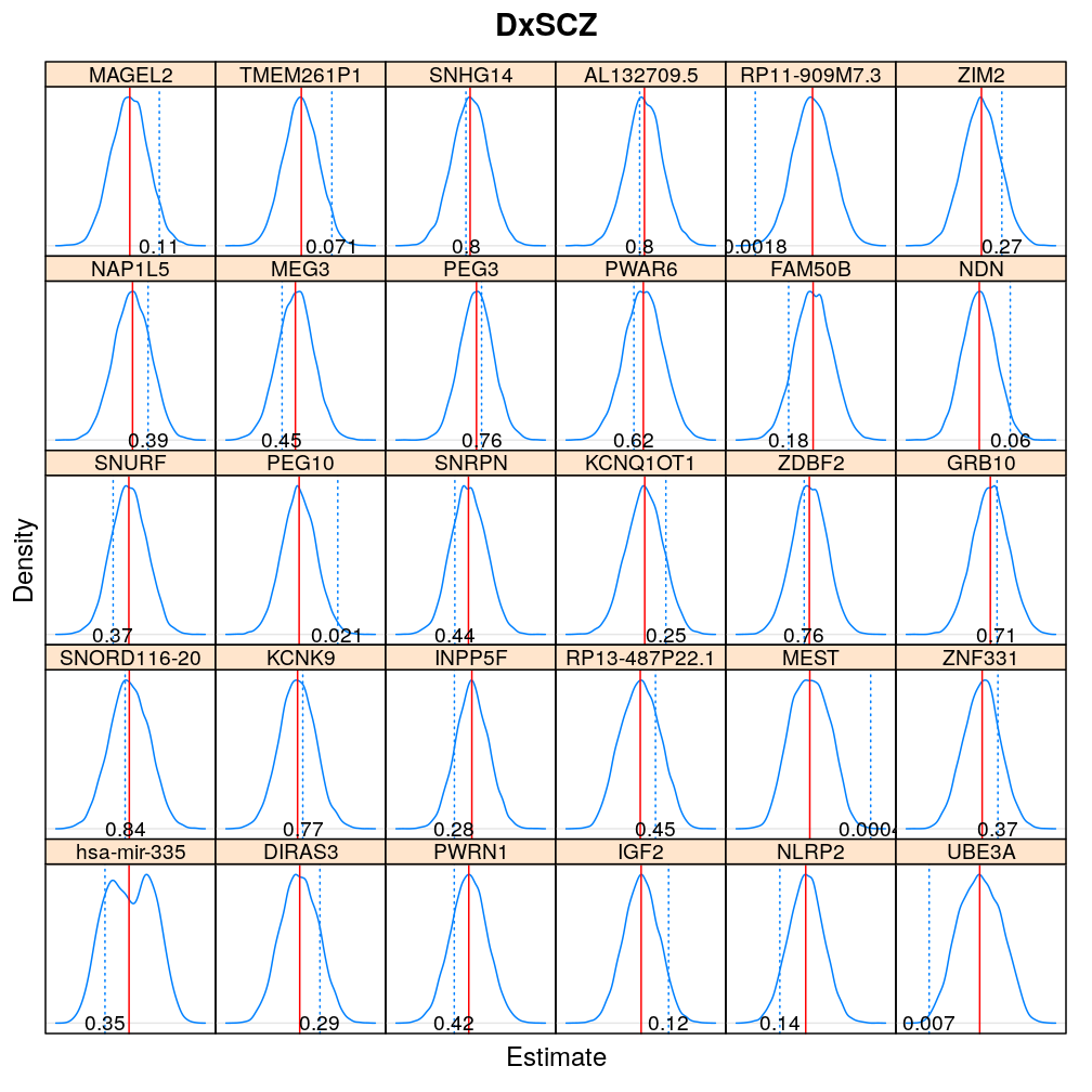
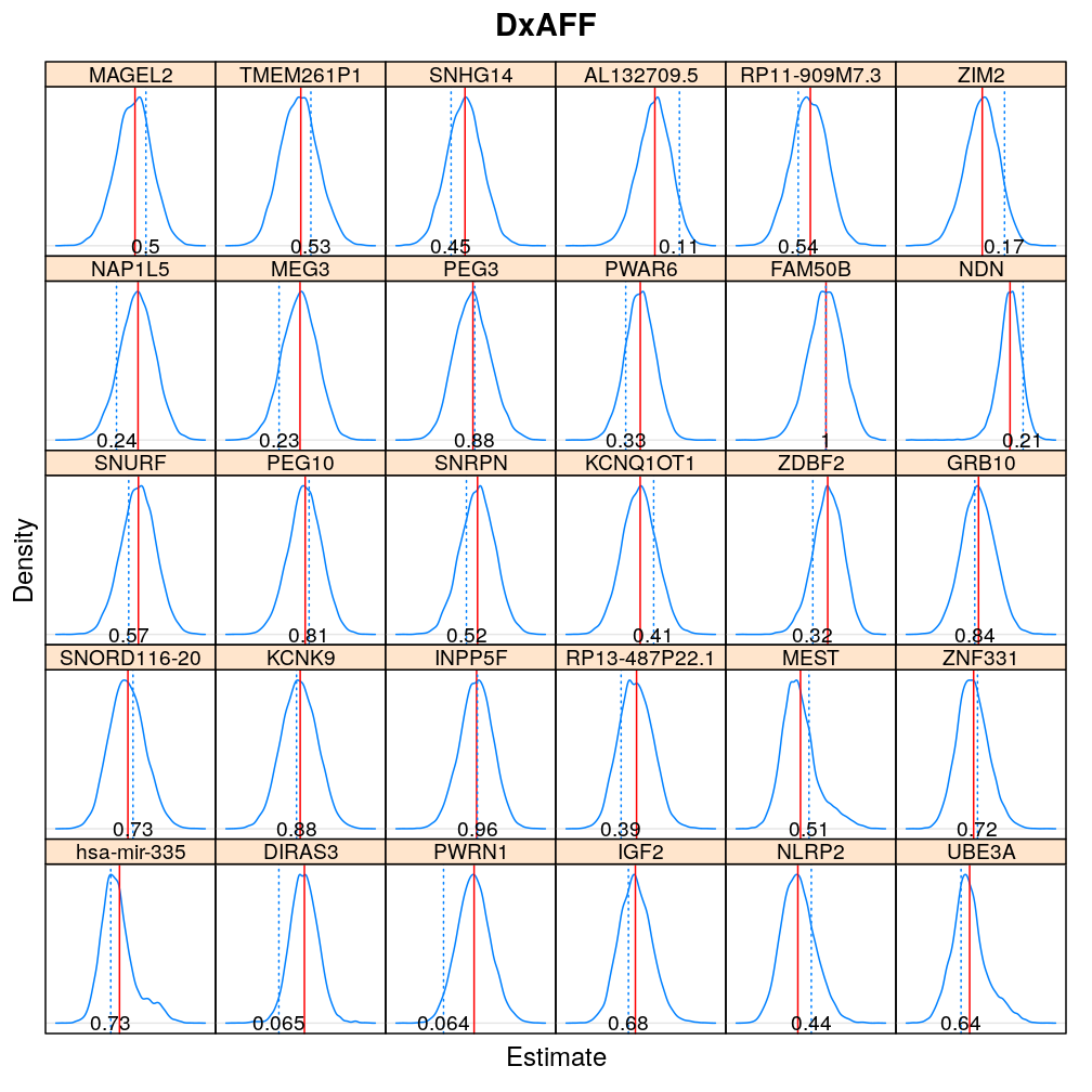
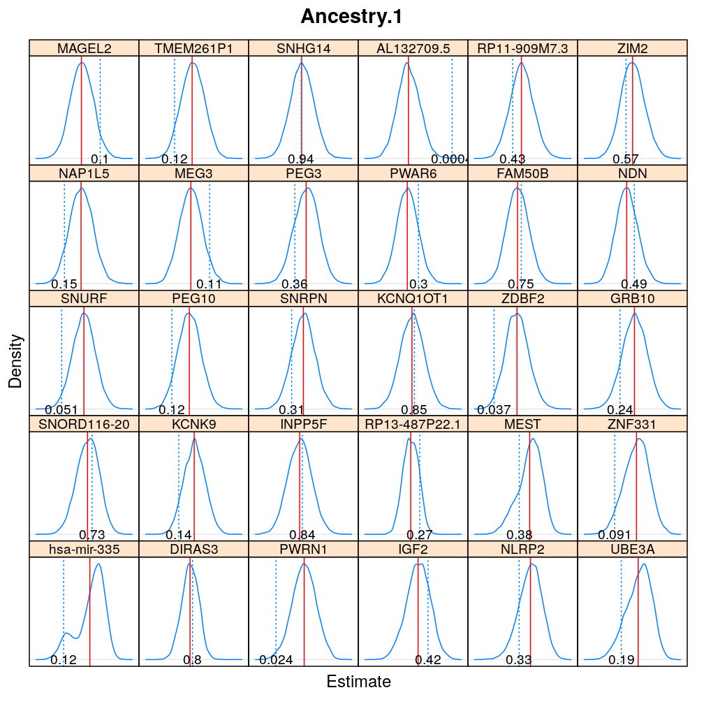
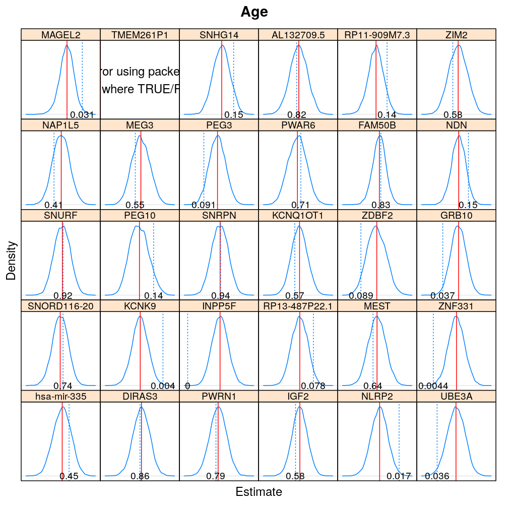
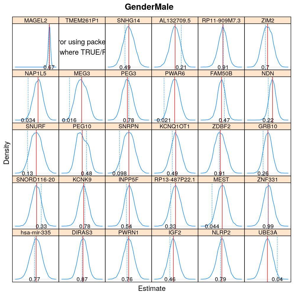
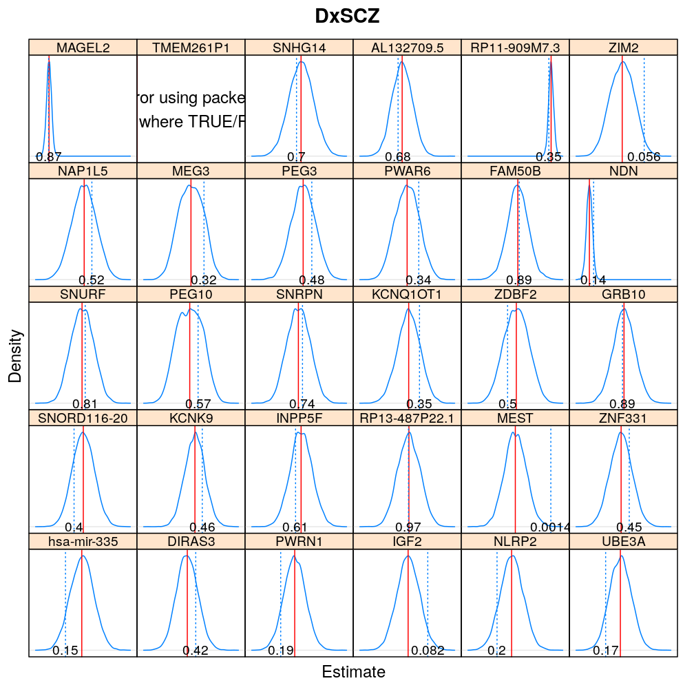
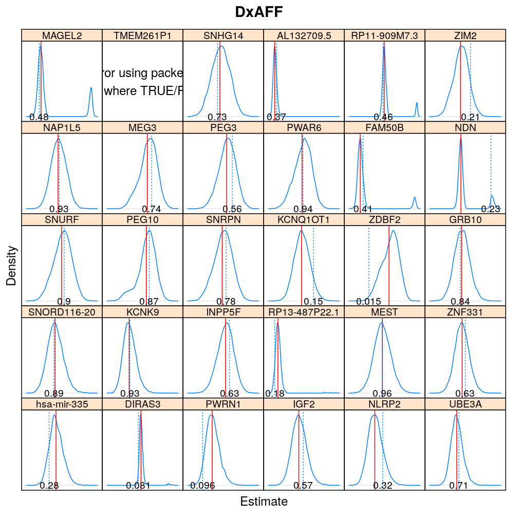
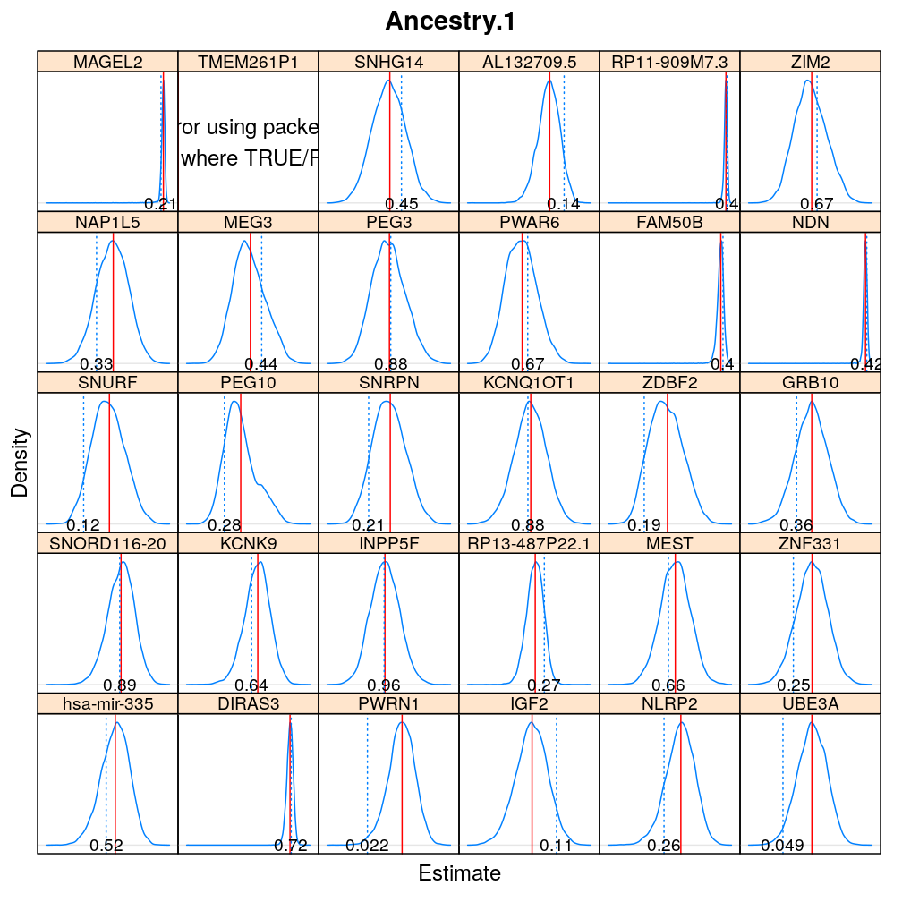
The expressions above obtain the null distribution of regression coefficients for the selected predictor(s) Age, Gender, Dx, Ancestry.1 under the selected model(s) wnlm.Q, logi.S based on 10⁴ permutations. Each panel within a plot shows a red vertical zero line of the null hypothesis $\beta_j = 0$ , the null distribution as probability density (solid blue line) based on the permutations, and the corresponding p-value (dotted blue line and number on the bottom).

Under wnlm.Q

beta0densityplot("Age", mtype = "wnlm.Q")

plot of chunk beta-age-null-wnlm-Q

plot of chunk beta-gender-null-wnlm-Q

plot of chunk beta-dx-scz-wnlm-Q

plot of chunk beta-dx-aff-wnlm-Q

plot of chunk beta-ancestry-1-null-wnlm-Q

Under logi.S

plot of chunk beta-age-null-logi-S

plot of chunk beta-gender-null-logi-S

plot of chunk beta-dx-scz-logi-S

plot of chunk beta-dx-aff-logi-S

plot of chunk beta-ancestry-1-null-logi-S

Comparison to p-values from t-distribution

The calculations and the plot below compare the p-values from the permutations to those based on the theoretical t-distribution of the statistic. Comparing these results to those from model checking reveals that the two approaches to p-value calculation agree (fall near the gray diagonal on the plots) as long as the model fits the data well. Otherwise the t-distribution based approach tends to produce much lower p-values and therefore exaggerate the significance that $\beta_j\neq 0$ .

source("2016-10-03-permutation-test.R")

M <- do.all.fits(Z = Y[gene.ids], G = E, preds = e.vars, sel.models = sel.models)
cf <- unlist(sapply(e.vars, function(e.v) predictor2coefs(M[[c(1, 1)]], e.v)))
both.p.val <-
    do.call(rbind,
            lapply(sel.models, function(mtype)
                   do.call(rbind,
                           lapply(cf, function(coef)
                                  do.call(rbind,
                                          lapply(gene.ids,
                                                 function(g) get.both.p.vals(mtype = mtype, gene = g, coef = coef, M = M, B = Betas)))))))

Adjust p-values of 0 to 10^-4, which is the reciprocal of the number of permutations. Without this adjustment these p-values couldn’t be plotted on a logarithmic scale.

both.p.val[with(both.p.val, ! is.na(p.val.perm) & p.val.perm == 0), "p.val.perm"] <- 1 / n.perm

pvalplot.genes.as.panels(both.p.val, ylim = c(-1, 15))

plot of chunk p-val-tdist-vs-perm

Filtering for poor fit

This filtering is based on earlier decisions on the goodness of fit of logi.S, which is stored in results/model-checking.csv.

both.p.val <- cbind(both.p.val, logi.S.OK <- read.csv("../../results/model-checking.csv", row.names = "gene")["logi.S.fit.OK"])
# set results to NA where logi.S fitted poorly
both.p.val[with(both.p.val, Model == "logi.S" & logi.S.fit.OK == FALSE), c("Estimate", "p.val.t.dist", "p.val.perm")] <- NA

Repeat the previous plot with the filtered results:

pvalplot.genes.as.panels(both.p.val, ylim = c(-1, 15))

plot of chunk p-val-tdist-vs-perm-filt

Equal x and y scaling (isometric):

plot of chunk p-val-tdist-vs-perm-filt-iso

Figures for manuscript

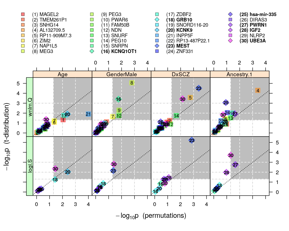
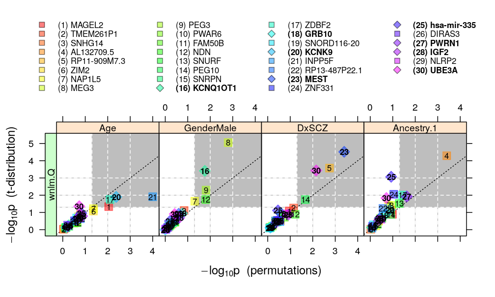
Figure for manuscript showing p-values calculated from both approaches (theory: t-distribution, and permutation test) and under both models (wnlm.Q and, when the fit was OK, also logi.S). The plotting symbols are color coded according to gene rank (rainbow, red to violet). The plotting symbols also display the rank with numbers, see the key on the top. Genes acceptably fitted by both models are distinguished with a diamond symbol and bold font from those that could be fitted only by wnlm.Q. Gray rectangle shows the decision rule, which rejects the null hypothesis if the p-value is smaller than 0.05 given both the t-distribution and the permutation-based test.

plot of chunk p-values

Leave logi.S out and show results only under wnlm.Q:

plot of chunk p-values-wnlm-Q

Summarizing results

Bringing results to long format and annotating significance with stars

v.names <- c("Estimate", "p.val.t.dist", "p.val.perm")
mtypes <- c("wnlm.Q", "logi.S")
varying <- lapply(c(v.names), function(v) sapply(mtypes, function(m) paste0(v, ".", m)))
both.p.val.w <-
    reshape(both.p.val, direction = "wide", varying = varying, v.names = v.names,
            timevar = "Model", times = mtypes, idvar = c("Gene", "Coefficient"))
stars <- data.frame(sapply(varying.p <- unlist(varying[-1])[c(1, 3, 2, 4)],
                           function(v) annotate.signif(both.p.val.w[[v]])))
names(stars) <- paste0(varying.p, ".*")
both.p.val.w <- cbind(both.p.val.w[2:1], stars, both.p.val.w[-1 * 2:1])

Aggregation

Aggregating significant findings over all four combinations of p-value calculation methods $v \in \{\mathrm{t.dist}, \mathrm{perm}\}$ and model types $y \in \{\mathrm{wnlm.Q}, \mathrm{logi.S}\}$ using the following rules

under a given model type $y$ take parameter–gene pairs $(j,g) \, \mid \, y$ for which $p_{jg}^{\mathrm{t.dist}, y} < 0.05 \; \mathrm{AND} \;p_{gj}^{\mathrm{perm}, y} < 0.05$
take if in the previous step
- either $(j,g) \, \mid \, \mathrm{wnlm.Q}$ or $(j,g) \, \mid \, \mathrm{logi.S}$ was taken
- both $(j,g) \, \mid \, \mathrm{wnlm.Q}$ and $(j,g) \, \mid \, \mathrm{logi.S}$ were taken

This means that we have the rules either and both, which correspond to a less and more stringent condition, respectively. These result in two corresponding sets of pairs, $\{(j,g) \, \mid \, \mathrm{either}\} \supseteq \{(j,g) \, \mid \, \mathrm{both}\}$ . (We also have the rules wnlm.Q and logi.S, which do not use aggregation over model types, and cannot be ordered in terms of stringency. Also, $\{(j,g) \, \mid \, \mathrm{wnlm.Q}\} \nsupseteq \{(j,g) \, \mid \, \mathrm{logi.S}\}$ and $\{(j,g) \, \mid \, \mathrm{wnlm.Q}\} \nsubseteq \{(j,g) \, \mid \, \mathrm{logi.S}\}$ in general).

The following code implements these rules.

is.signif <-
    list(wnlm.Q =
             with(both.p.val.w, p.val.t.dist.wnlm.Q < 5e-2 & p.val.perm.wnlm.Q < 5e-2 &
                  Coefficient %in% c("Age", "GenderMale", "Ancestry.1", "DxSCZ")),
         logi.S =
             with(both.p.val.w, logi.S.fit.OK & p.val.t.dist.logi.S < 5e-2 & p.val.perm.logi.S < 5e-2 &
                  Coefficient %in% c("Age", "GenderMale", "Ancestry.1", "DxSCZ")))
is.signif$either <- with(is.signif, wnlm.Q | logi.S)
is.signif$both <- with(is.signif, wnlm.Q & logi.S)

The pairs $\{(j,g) \, \mid \, x\}$ (where $x \in \{\mathrm{wnlm.Q}, \mathrm{logi.S}, \mathrm{either}, \mathrm{both}\}$ ) can be presented in two sensible ways: a gene-centric and a coefficient-centric way.

The gene-centric way lists, for each gene, all the significantly associated coefficients:

signif.gene.effects <-
    lapply(is.signif,
           function(s)
               sapply(split(x <- both.p.val.w[s, c("Gene", "Coefficient")][ with(both.p.val.w[is.signif$either, ], order(Gene, Coefficient)), ], x$Gene, drop = TRUE),
                      function(g) toString(g$Coefficient)))
signif.gene.effects

## $wnlm.Q
##            MAGEL2        AL132709.5      RP11-909M7.3            NAP1L5 
##             "Age"      "Ancestry.1"           "DxSCZ"      "GenderMale" 
##              MEG3              PEG3               NDN             PEG10 
##      "GenderMale"      "GenderMale"      "GenderMale"           "DxSCZ" 
##          KCNQ1OT1             ZDBF2             KCNK9            INPP5F 
##      "GenderMale" "Age, Ancestry.1"             "Age"             "Age" 
##              MEST             PWRN1             UBE3A 
##           "DxSCZ"      "Ancestry.1"           "DxSCZ" 
## 
## $logi.S
##                         KCNK9                          MEST 
##                         "Age"           "GenderMale, DxSCZ" 
##                         PWRN1                         UBE3A 
##                  "Ancestry.1" "Ancestry.1, Age, GenderMale" 
## 
## $either
##                               MAGEL2                           AL132709.5 
##                                "Age"                         "Ancestry.1" 
##                         RP11-909M7.3                               NAP1L5 
##                              "DxSCZ"                         "GenderMale" 
##                                 MEG3                                 PEG3 
##                         "GenderMale"                         "GenderMale" 
##                                  NDN                                PEG10 
##                         "GenderMale"                              "DxSCZ" 
##                             KCNQ1OT1                                ZDBF2 
##                         "GenderMale"                    "Age, Ancestry.1" 
##                                KCNK9                               INPP5F 
##                                "Age"                                "Age" 
##                                 MEST                                PWRN1 
##                  "GenderMale, DxSCZ"                         "Ancestry.1" 
##                                UBE3A 
## "Age, GenderMale, DxSCZ, Ancestry.1" 
## 
## $both
##        KCNK9         MEST        PWRN1 
##        "Age"      "DxSCZ" "Ancestry.1"

The coefficient-centric way lists, for each coefficient, all the significantly associated genes:

signif.effect.genes <-
    lapply(is.signif,
           function(s)
               sapply(split(x <- both.p.val.w[s, c("Gene", "Coefficient")][ with(both.p.val.w[is.signif$either, ], order(Coefficient, Gene)), ], x$Coefficient, drop = TRUE),
                      function(g) toString(g$Gene)))
signif.effect.genes

## $wnlm.Q
##                                 Age                          GenderMale 
##      "MAGEL2, ZDBF2, KCNK9, INPP5F" "NAP1L5, MEG3, PEG3, NDN, KCNQ1OT1" 
##                               DxSCZ                          Ancestry.1 
##  "RP11-909M7.3, PEG10, MEST, UBE3A"          "AL132709.5, ZDBF2, PWRN1" 
## 
## $logi.S
##            Age     GenderMale          DxSCZ     Ancestry.1 
## "KCNK9, UBE3A"  "MEST, UBE3A"         "MEST" "PWRN1, UBE3A" 
## 
## $either
##                                              Age 
##            "MAGEL2, ZDBF2, KCNK9, INPP5F, UBE3A" 
##                                       GenderMale 
## "NAP1L5, MEG3, PEG3, NDN, KCNQ1OT1, MEST, UBE3A" 
##                                            DxSCZ 
##               "RP11-909M7.3, PEG10, MEST, UBE3A" 
##                                       Ancestry.1 
##                "AL132709.5, ZDBF2, PWRN1, UBE3A" 
## 
## $both
##        Age      DxSCZ Ancestry.1 
##    "KCNK9"     "MEST"    "PWRN1"

Writing results to files

write.csv(both.p.val, "../../results/regr-coefs.csv", row.names = FALSE)
write.csv(both.p.val.w, "../../results/regr-coefs-w.csv", row.names = FALSE)
invisible(lapply(names(signif.gene.effects),
                 function(x) write.csv(data.frame(Gene = names(y <- signif.gene.effects[[x]]), Coefficient = y), file = paste0("../../results/signif-gene-effects-", x, ".csv"), row.names = FALSE)))
invisible(lapply(names(signif.effect.genes),
                 function(x) write.csv(data.frame(Gene = names(y <- signif.effect.genes[[x]]), Coefficient = y), file = paste0("../../results/signif-effect-genes-", x, ".csv"), row.names = FALSE)))

Lab Notebook

Author of notebook: Attila Gulyás-Kovács, Chess Lab, Mount Sinai School of Medicine. Related publication: Nat Commun. 2018 Jul 25;9(1):2914